Multivariate Non-parametric Kernel Density. Estimation for Visual Surveillance. Alireza Tavakkoli, Mircea Nicolescu, and George Bebis. Computer Vision ...
Automatic Robust Background Modeling Using Multivariate Non-parametric Kernel Density Estimation for Visual Surveillance Alireza Tavakkoli, Mircea Nicolescu, and George Bebis Computer Vision Laboratory, University of Nevada, Reno, NV 89557 Abstract. The final goal for many visual surveillance systems is automatic understanding of events in a site. Higher level processing on video data requires certain lower level vision tasks to be performed. One of these tasks is the segmentation of video data into regions that correspond to objects in the scene. Issues such as automation, noise robustness, adaptation, and accuracy of the model must be addressed. Current background modeling techniques use heuristics to build a representation of the background, while it would be desirable to obtain the background model automatically. In order to increase the accuracy of modeling it needs to adapt to different parts of the same scene and finally the model has to be robust to noise. The building block of the model representation used in this paper is multivariate non-parametric kernel density estimation which builds a statistical model for the background of the video scene based on the probability density function of its pixels. A post processing step is applied to the background model to achieve the spatial consistency of the foreground objects.
1
Introduction
An important ultimate goal of automated surveillance systems is to understand the activities in a site, usually monitored by fixed cameras and/or other sensors. This enables functionalities such as automatic detection of suspicious activities, site security, etc. The first step toward automatic recognition of events is to detect and track objects of interest in order to make higher level decisions on their interactions. One of the most widely used techniques for detection and tracking of objects in the video scene is background modeling. The most commonly used feature in background modeling techniques is pixel intensity. In a video with a stationary background (i.e. video taken by a fixed camera) deviations of pixel intensity values over time can be modeled as noise by a Gaussian distribution function, N (0, σ 2 ). A simplistic background modeling technique is to calculate the average of intensity at every pixel position, find the difference at each frame with this average and threshold the result. Using an adaptive filter this model follows gradual changes in the scene illumination, as shown in [1]. Kalman filtering is also used in [2], [3] and [4]. Also a linear prediction using Wiegner Filter is used in [5]. In some particular environments with changing parts of background, such as outdoor environments with waving trees, surface of water, etc., the background is G. Bebis et al. (Eds.): ISVC 2005, LNCS 3804, pp. 363–370, 2005. c Springer-Verlag Berlin Heidelberg 2005 �
364
A. Tavakkoli, M. Nicolescu, and G. Bebis Table 1. Comparison of methods
Method Color Independency Automatic Threshold Spatial Consistency Parametric Yes No No Non-parametric No No No Proposed Yes Yes Yes
not completely stationary. For these applications mixture of Gaussians has been proposed in [6], [7] and [8]. In order to find the parameters of the mixture of Gaussians, the EM algorithm is used while the adaptation of parameters can be achieved by using an incremental version of the EM algorithm. Another approach to model variations in the background model is to represent these changes as different states, corresponding to different environments; such as lights on/off, night/day, sunny/cloudy. For this purpose Hidden Markov Models (HMM) have been used in [9] and [10]. Edge features are also used as a tool to model the background in [11] and [12] based on comparing edges and fusion of intensity and edge information, respectively. Also block features are used in [13] and [14]. One of the most successful approaches in background subtraction is proposed in [15]. Here the background representation is drawn by estimating the probability density function of each pixel in the background model. In this paper, the statistical background model is built by multi-variate nonparametric kernel density estimation. Then the model is used to automatically compute a threshold for the probability of each pixel in the incoming video frames. Finally a post processing stage makes the model robust to salt-andpepper noise that may affect the video. Table 1 shows a comparison between the traditional parametric and non-parametric statistical representation techniques and our proposed method that addresses the above issues. The rest of this paper is organized as follows. In Section 2 the proposed algorithm is presented and Section 3 describes our bi-variate approach to the density estimation. In Section 4 we discuss our proposed automatic selection of covariance matrix and suitable thresholds for each pixel in the scene. In Section 5 the noise reduction stage of the algorithm is presented by enforcing spatial consistency. Section 6 discusses our adaptation approach and in Section 7 experimental results of our algorithm are compared to traditional techniques. Section 8 summarizes our approach and discusses future extensions of this work.
2
Overview of the Proposed Algorithm
We propose an automatic and robust background modeling based on multivariate non-parametric kernel density estimation. The proposed method has three major parts. In the training stage, parameters of the model are trained and estimated for each pixel, based on their values in the background training frames. In the next stage, classification step, the probability that a pixel belongs to the background in every frame is estimated using our bi-variate density estimation. Then pixels are marked as background or foreground based on their probability
Automatic Robust Background Modeling
365
Fig. 1. Our Proposed Background Modeling Algorithm
values. The final stage of our proposed algorithm removes those pixels that do not belong to a true foreground region, but due to strong noise are selected as foreground. In Fig. 1, the proposed algorithm is presented. The automation is achieved in the training stage, which uses the background model to train a single class classifier based on the training set for each pixel. Also by using step 2.2., we address the salt-and-pepper noise issue in the video.
3
Bi-variate Kernel Density Estimation
In [15], the probability density of a pixel being background is calculated by: � �2 � � N d 1 1 �� 1 xtj − xij � P r(xt ) = × exp − (1) N i=1 j=1 2πσ 2 2 σj j
As mentioned in Section 2, the first step of the proposed algorithm is the bivariate non-parametric kernel density estimation. The reason for using multivariate kernels is that our observations on the scatter plot of color and normalized chrominance values, introduced in [15], show that these values are not independent. The proposed density estimation can be achieved by:
N 1 1 � 1 T −1 � P r(xt ) = exp − (xt − xi ) Σ (xt − xi ) N i=1 (2π)2 |Σ| 2 where x = [Cr , Cg ], Cr =
R R+G+B
and Cg =
G R+G+B .
(2)
366
A. Tavakkoli, M. Nicolescu, and G. Bebis
(a) Scatter Plot
(b) Univariate
(c) Bivariate
(d) 3D illustration
Fig. 2. Red/Green chrominance scatter plot of an arbitrary pixel
In equation (2) xt is the chrominance vector of each pixel in frame number t and xi is the chrominance vector of the corresponding pixel in frame i of the background model. Also, Σ is the covariance matrix of the chrominance components. As it is shown in [16], kernel bandwidths are not important if the number of training samples reaches infinity. In this application, we have limited samples for each pixel, so we need to automatically select a suitable kernel bandwidth for each pixel. By using the the covariance matrix of the training data for each pixel, bandwidths are automatically estimated. In Fig. 2, the scatter plot of red and green chrominance values of an arbitrary pixel shows that these values are not completely independent, and follow some patterns, as shown in Fig. 2(a). As expected the contours of simple traditional model are horizontal or vertical ellipses, while the proposed method gives more accurate boundaries with ellipses in the direction of the scatter of chrominance values. Fig 2(c) shows the constant level contours of the estimated probability density function using the multi-variate probability density estimation from equation (2). In Fig. 2(d) a three dimensional illustration of the estimated probability density function is shown. The only parameters that we have to estimate in our framework are the probability threshold Th, to discriminate between foreground and background pixels, and the covariance matrix Σ.
4
The Training Stage
As mentioned in Section 2, in order to make the background modeling technique automatic, we need to select two parameters for each pixel: the covariance matrix Σ in equation (2) and the threshold Th. 4.1
Automatic Selection of Σ
Theoretically, the summation in Equation (2) will converge to the actual underlying bi-variate probability density function as the number of background frames reaches infinity. Since in practical applications, one can not use infinite number of background frames to estimate the probability, there is a need to find a suitable value of Σ parameters for every pixel in the background model. In order to find the suitable choice of Σ, for each pixel we first calculate the deviation of successive chrominance values for all pixels in the background
Automatic Robust Background Modeling
367
model. Then the covariance matrix of this population is used as the Σ value. As a result the scene independent probability density of each chrominance value is estimated. In the case of a multi-modal scatter plot, observations that do not consider the successive deviations show global deviation not the local modes in the scatter plot. 4.2
Automatic Selection of Threshold
In traditional methods, both parametric and non parametric, the same global threshold for all pixels in the frame is selected, heuristically. The proposed method automatically estimates local thresholds for every pixel in the scene. In our application we used the training frames as our prior knowledge about the background model. If we estimate the probability of each pixel in the background training data, these probabilities should be high. By estimating the probability for each pixel in all of the background training frames we have a fluctuating function shown in Fig. 3.
Fig. 3. Estimated probabilities of a pixel in the background training frame
We propose a probabilistic threshold training stage where we compute successive deviation of the estimated probabilities for each pixel in the training frames. The probability density function of this population is a zero mean Gaussian distribution. Then we calculate the 95 percentile of this distribution and use it as the threshold for that pixel.
5
Enforcing Spatial Consistency
Our observations show that if a pixel is selected as foreground due to strong noise, it is unlikely that the neighboring pixels, both in time and space, are also affected by this noise. To address this issue, instead of using the threshold directly on the estimated probability of pixels in the current frame, we calculate the median of probabilities of pixels in the 8-connected region surrounding current pixel. Then the threshold is applied on the median probability, instead of the actual one. Finally, a connected component analysis is used to remove the remaining regions with a very small area.
6
Adaptation to Gradual and Sudden Changes in Illumination
In the proposed method we use two different types of adaptation. To make the system adaptable to gradual changes in illumination, we replace pixels in the
368
A. Tavakkoli, M. Nicolescu, and G. Bebis
oldest background frame with those pixels belonging to the current background mask. To make the algorithm adaptable to sudden changes in the illumination, we track the area of the detected foreground objects. Once we detect a sudden change in their area, the detection part of the algorithm is suspended. Current frames replace the background training frames, and based on the latest reliable foreground mask, the foreground objects are detected. Because the training stage of the algorithm is very time consuming the updating stage is is performed every few frames, depending on the rate of the changes and the processing power.
7
Experimental Results
In this section, experimental results of our proposed method are presented and compared to the existing methods. Fig. 4 and Fig. 5 show frame number 380 of the ”jump” and 28 of ”rain” video sequences, respectively. The sequence in Fig. 4(a) poses significant challenges due to the moving tree branches, which makes the detection of true foreground (the two persons) very difficult. Rain in Fig. 5(a) makes this task very difficult. Results of [15] and the proposed method for these two video sequences are shown in Fig. 4 and Fig. 5 (b) and (c), respectively. Fig. 6 shows the performance of the proposed method on some challenging scenes. In Fig. 6(a) moving branches of trees as well as waving flags and strips pose difficulties in detection of foreground. Fluctuation of illumination
(a)
(b)
(c)
Fig. 4. Foreground masks selected from frame number 380 of the ”jump” sequence: (a) Frame number 380. (b) Foreground masks detected using [15] and (c) using our proposed algorithm.
(a)
(b)
(c)
Fig. 5. Foreground masks selected from frame number 28 of the ”rain” sequence: (a) Frame number 28. (b) Foreground masks detected using [15] and (c) using our proposed algorithm.
Automatic Robust Background Modeling
(a)
(d)
(b)
(e)
369
(c)
(f)
Fig. 6. Foreground masks selected from some difficult video scences using our proposed algorithm
in Fig. 6(b) due to flickering of monitor and light make this task difficult and waves and rain on the surface of water is challenging in Fig. 6(c). Results of the proposed algorithm for these scenes are presented in Fig. 6(d), (e) and (f), respectively. The only time consuming part of the proposed algorithm is the training part, which is performed every few frames and does not interfere with the detection stage. Automatic selection of thresholds is another advantage of the proposed method.
8
Conclusions and Future Work
In this paper we propose a fully automatic and robust technique for background modeling and foreground detection based on multivariate non-parametric kernel density estimation. In the training stage, the thresholds for the estimated probability of every pixel in the scene is automatically trained. In order to achieve robustness and accurate foreground detection, we also propose a spatial consistency processing step. Further extensions of this work include using other features of the image pixels, such as their HSV or L,a,b values. Also spatial and temporal consistency can be achieved by incorporating the position of pixels and their time index as additional features.
Acknowledgements This work was supported in part by a grant from the University of Nevada Junior Research Grant Fund and by NASA under grant # NCC5-583. This support does not necessarily imply endorsement by the University of research conclusions.
370
A. Tavakkoli, M. Nicolescu, and G. Bebis
References 1. Wern, C., Azarbayejani, A., Darrel, T., Petland, A.P.: Pfinder: real-time tracking of human body. IEEE Transactions on PAMI (1997) 2. Karman, K.P., von Brandt, A.: Moving object recognition using an adaptive background memory. Time-Varying Image Processing and Moving Object Recognition, Elsevier (1990) 3. Karman, K.P., von Brandt, A.: Moving object segmentation based on adaptive reference images. Signal Processing V: Theories and Applications, Elsevier Science Publishers B.V., (1990) 4. Koller, D., Weber, J., Haung, T., Malik, J., Ogasawara, G., Roa, B., Russel, S.: Toward robust automatic traffic scene analysis in real-time. In: ICPR. (1994) 126– 131. 5. Toyama, K., Krumm, J., Brumitt, B., Meyers, B.: Wallflower: Principles and practice of background maintenance. In: ICCV. (1999) . 6. Grimson, W., Stauffer, C., Romano, R.: Using adaptive tracking to classify and monitor activities in a site. CVPR, (1998) 7. Grimson, W., Stauffer, C.: Adaptive background mixture models for real-time tracking. CVPR, (1998) 8. Friedman, N., Russel, S.: Image segmentation in video sequences: A probabilistic approach. Uncertainty in Artificial Intelligence, (1997) 9. J. Rittscher, J. Kato, S.J., Blake, A.: A probabilistic background model for tracking. In: 6th European Conf. on Computer Vision. Volume 2. (2000) 336–350. 10. B. Stenger, V. Ramesh, N.P.F.C., Bouthman, J.: Topology free hidden markov models: Application to background modeling. In: ICCV. (2001) 294–301. 11. Yang, Y., Levine, M.: The background primal sketch: An approach for tracking moving objects. Machine Vision and Applications, (1992) 12. S. Jabri, Z. Duric, H.W., Rosenfled, A.: Detection and location of people video images using adaptive fusion of color and edge information. In: ICPR. (2000) . 13. Y. Hus, H.H.N., Rekers, G.: New likelihood test methods for change detection in image sequences. Computer Vision and Image Processing, (1984) 14. Matsuyama, T., Ohya, T., Habe, H.: Background subtraction for non-stationary scenes. In: 4th Asian Conf. on Computer Vision. (2000) 662–667. 15. A. Elgammal, R. Duraiswami, D.H., Davis, L.S.: Background and foreground modeling using nonparametric kernel density estimation for visual surveillance. (In: IEEE) 1151–1163. 16. R. O. Duda, D.G.S., Hart, P.E.: Pattern classification. 2nd edn. Wiley John & Sons (2000)