Manifold Learning and its Applications: Papers from the AAAI Fall Symposium (FS-09-04)
Robust Laplacian Eigenmaps Using Global Information ∗ Shounak Roychowdhury
Joydeep Ghosh
ECE University of Texas at Austin, Austin, TX email:
[email protected]
ECE University of Texas at Austin, Austin, TX email:
[email protected]
Abstract
Space Alignment (Zhang and Zha 2002). Belkin and Niyogi in (Belkin and Niyogi 2003) proposed Laplacian Eigenmaps (LEM), a method that approximates the Laplace-Beltrami Operator which is able to capture the properties of any Riemaniann manifold. Donoho and Grimes have proposed a method similar to LEM using Hessian Maps (Donoho and Grimes 2003). Recently Shaw and Jebara (Shaw and Jebara 2009) proposed an embedding method that preserves the structure of the data.
The Laplacian Eigenmap is a popular method for non-linear dimension reduction and data representation. This graph based method uses a Graph Laplacian matrix that closely approximates the Laplace-Beltrami operator which has properties that help to learn the structure of data lying on Riemaniann manifolds. However, the Graph Laplacian used in this method is derived from an intermediate graph that is built using local neighborhood information. In this paper we show that it possible to encapsulate global information represented by a Minimum Spanning Tree on the data set and use it for effective dimension reduction when local information is limited. The ability of MSTs to capture intrinsic dimension and intrinsic entropy of manifolds has been shown in a recent study. Based on that result we show that the use of local neighborhood and global graph can preserve the locality of the manifold. The experimental results validate the simultaneous use of local and global information for non-linear dimension reduction.
The motivation of our work derives from our experimental observations that when the graph used in LEM is not wellconstructed (either it has lot of isolated vertices or there are islands of subgraphs) the data is difficult to interpret after a dimension reduction. This paper discusses how global information can be used in addition to local information in the framework of Laplacian Eigenmaps to address such situations. We make use of an interesting result by Costa and Hero that shows that Minimum Spanning Tree on a manifold can reveal its intrinsic dimension and entropy (Costa and Hero 2004). In other words, it implies that MSTs can capture the underlying global structure of the manifold if it exists. We use this finding to extend the dimension reduction technique using LEM to exploit both local and global information.
Introduction Dimensionality reduction is an important process that is often required to understand the data in more tractable and humanly comprehensible way. This process has been extensively studied in terms of linear methods such as Principal Component Analysis (PCA), Independent Component Analysis (ICA), Factor Analysis etc. (Hastie, Tibshirani, and Friedman 2001). However, it has been noticed that many high dimensional data such as a series of related images, lie on a manifold (Seung and Lee 2000) and are not scattered throughout the feature space. This particular observation has motivated many researchers to develop dimension reduction algorithms that try to learn an embedded manifold in the high dimensional space. ISOMAP (Tenenbaum, de Silva, and Langford 2000) looks tries to learn the manifold by exploring geodesic distances. Locally Linear Embedding (LLE) is an unsupervised learning method based on global and local optimization (Saul, Roweis, and Singer 2003). Zhang et. al. proposed a method of finding Principal Manifolds using Local Tangent
LEM depends on the Graph Laplacian matrix and so does our work. Fiedler initially proposed the Graph Laplacian matrix as a means to comprehend the notion of algebraic connectivity of a graph (Fiedler 1973). Merris has extensively discussed the wide variety of properties of the Laplacian matrix of a graph such as invariance, on various bounds and inequalities, extremal examples and constructions etc. in his survey (Merris 1994). A broader role of the Laplacian matrix can be seen in Chung’s book on Spectral Graph Theory (Chung 1997). The second section touches on the Graph Laplacian matrix. The role of global information in manifold learning is then presented, followed by our proposed approach of augmenting LEM by including global information about the data. Experimental results confirm that global information can indeed help when the local information is limited for manifold learning.
∗ This research was supported in part by NSF (Grant IIS0705836). c 2009, Association for the Advancement of Artificial Copyright Intelligence (www.aaai.org). All rights reserved.
42
Graph G
Graph Laplacian In this section we will briefly review the definitions of a Graph Laplacian matrix and Laplacian of Graph Sum.
Definitions Let us consider a weighted graph G = (V, E), where V = V (G) = {v1 , v2 , ..., vn } is the set of vertices (also called vertex set) and E = E(G) = {e1 , e2 , ..., en } is the set of edges (also called edge set). The weight w function is defined as w : V × V → ℜ such that w(vi , vj )=w(vj , vi )=wij . Definition 1: The Laplacian (Fiedler 1973) of a graph without loops of multiple edges is defined as the following: dvi if vi = vj L(G) = −1 if vi are vj adjacent, (1) 0 Otherwise.
80
60
60
40
40
20
20 40
60
80
20
40
60
80
J=G⊕H 80 60 40 20 20
40
60
80
Figure 1: The top-left figure shows a graph G; top-right figure shows a MST graph H; and the bottom-left figure shows the Graph Sum J = G ⊕ H. Note how the graphs superimpose on each other to form a new graph.
(2) matrix of the summed graph. Let G and H be two graphs of order n, and the new summed graph be denoted by J as shown in Figure 1. Furthermore, let AG , AH , and AJ be the adjacency of each graph respectively. Then
A definition by Chung (see (Chung 1997)) – which is given below – generalizes the Laplacian by adding the weights on the edges of the graph. It can be viewed as Weighed Graph Laplacian. Simply, it is a difference between the diagonal matrix D and the W the weighted adjacency matrix. LW (G) = D − W,
80
20
Fiedler (Fiedler 1973) defined the Laplacian of a graph as symmetric matrix for regular graph, where A is an adjacency matrix (AT is the transpose of adjacency matrix), I is the identity matrix and n is the degree of the regular graph: L(G) = nI − A.
Graph H
J = G ⊕ H, and AJ = AG + AH .
(3)
From Definition 2, it is obvious that
where Pn the diagonal element in D is defined as dvi = j=1 w(vi , vj ). Definition 2: The Laplacian of weighted graph (operator) is defined as the following: dvi − w(vi , vj ) if vi = vj Lw (G) = −w(vi , vj ) if vi are vj connected (4) 0 otherwise.
Lw (J) = Lw (G) + Lw (H).
(5)
Global Information of Manifold Global information has not been used in manifold learning since it is widely believed that global information may capture unnecessary data (like ambient data points) that should be avoided when dealing with manifolds. However, some recent research results show that that it might be useful to to explore global information in a more constrained manner for manifold learning. Costa and Hero show that it is possible to use a Geodesic Minimum Spanning Tree (GMST) on the manifold to estimate the intrinsic dimension and intrinsic entropy of the manifold (Costa and Hero 2004). Costa and Hero showed in the following theorem that is possible to learn the intrinsic entropy and intrinsic dimension of a non-linear manifold by extending the BHH theorem (Beardwood, Halton, and Hammersley 1959), a well-known result in Geometric Probability.
Lw (G) reduces to L(G) when the edges have unit weights.
Laplacian of Graph Sum Here we are primarily interested in knowing how to derive Laplacian of a resultant graph derived from two different graphs of same order (on a given data set). In fact we are superimposing two graphs having same set of vertices together to form a new graph. We do graph fusion as we are interested in combining local-neighborhood graph and a global graph which we will describe later on. Harary in (Harary 1990) introduced a graph operator called Graph Sum, the operator is denoted by ⊕ : G × H → J, to sum up two graphs of the same order (|V (G)| = |V (H)| = |V (J)|). The operator is quite simple – adjacency matrices of each graph are numerically added to form the adjacency
Theorem 1 (Generalization of BHH Theorem to Embedded manifolds: (Costa and Hero 2004)). Let M be a smooth compact m-dimensional manifold embedded in Rd through the diffeomorphism φ : Ω → M, and Ω ∈ Rd .
43
Assume 2 ≤ m ≤ d and 0 < γ < m. Suppose that Y1 , Y2 , ... are iid random vectors on M having a common density function f with respect to a Lebesgue measure µM on m M. Then the length functional TγR φ−1 (Yn ) of the MST spanning φ−1 (Yn ) satisfies the equation shown below in an almost sure sense:
Algorithm 1: Global Laplacian Eigenmaps (GLEM) Data: Data: Xn×p where n is the number of data points and p is the number of dimensions. k: number of fixed neighbors or ǫ − ball: using neighbors falling within a ball of radius ǫ, and 0 ≤ λ ≤ 1 Result: Low-dimensional subspace; Xn×m where n is the number of data points and m is then number of selected eigen-dimensions such that m ≪ p. 1 begin 2 Construct the graph GN N either by using local neighbor k or ǫ − ball. Construct the Adjacency Graph A(GN N ) of graph GN N . 3 Compute the weight matrix (WN N ) from the weights of the edges of graph GN N using the Heat Kernel function. 4 Compute Laplacian matrix L(GN N ) = DN N WN N /* DN N is the Diagonal Matrix of the NN Graph. */ 5 Construct the graph GMST . Construct the Adjacency Graph A(GMST ) of graph GMST . 6 Compute the weight matrix (WMST ) from the weights of the edges of graph GMST using the Heat Kernel function. 7 Compute Laplacian matrix L(GMST ) = DMST WMST /* DMST is the Diagonal Matrix of the MST Graph. */ 8 L(G) = L(GN N ) + λL(GMST ) 9 return the subspace Xn×m by selecting first m eigenvectors of L(G) 10 end
m
lim
n→∞
TγR φ−1 (Yn ) n
(d−1) d
=
d′ < m ∞ R T α β [det(Jφ Jφ )]f (x) µM d(y) a.s., d′ = m (6) m M 0 d′ > m where α = (m − γ)/m, and is always between 0 < α < 1, J is the Jacobian, and βm is a constant which depends on m. Based on the above theorem we use MST on the entire data set as a source of global information. For more details see (Costa and Hero 2004), and more background information see (Yukich 1998) and (Steele 1997). The basic principle of GLEM is quite straight forward. The objective function that is to be minimized is given by following (it is has the same flavor and notation used in (Belkin and Niyogi 2003)): X ||y(i) − y(j) ||22 (WijN N + WijMST ) i,j
=
tr(YT L(GN N )Y + YT L(GMST )Y)
(7)
T
=
tr(Y (L(GN N ) + L(GMST ))Y)
=
tr(YT L(J)Y).
where y(i) = [y1 (i), ..., ym (i)]T , and m is the dimension of embedding. WijN N and WijMST are weighted matrices of kNearest Neighbor graph and the MST graph respectively. In other words, we have arg min YT LY
where t > 0. Thereafter compute the MST graph GMST on the data set, and its Laplacian L(GMST ). Based on Laplacian Graph summation as described earlier, we now combine two graphs GN N and GMST by effectively adding their Laplacians L(GN N ) and L(GMST ).
(8)
Y YT DY=I
Experiments
such that Y = [y1 , y2 , ..., ym ] and y(i) is the mdimensional representation of ith vertex. The solutions to this optimization problem are the eigenvectors of the generalized eigenvalue problem
Here we show the results of our experiments conducted on two well-known manifold data sets: 1) S-Curve and 2) ISOMAP face data set (ISOMAP 2009) using LEM which uses the local neighborhood information, and GLEM which exploits local as well as global information of the manifold. For calculation of local neighborhood we use kN N method. The S-Curve data is shown in Fig.2 for reference. The MST on the S-Curve data is shown in Figure 3. The top figure shows the MST of data, while the bottom figure shows the embedding of the graph. Notice how the data is embedded in tree-like structure, yet the local information of the data is completely preserved. Figure 4 shows embedding of the ISOMAP face data set using the MST graph. We use a limited number of face images to clearly show the embedded structure, the data points are shown by ‘+’ in embedded space.
LY = ΛDY. The GLEM algorithm is described in Algorithm 1.
Laplacian Eigenmaps with Global Information In this section we describe our approach of using the global information of the manifold which is modeled as a MST. Similar to the LEM approach our method (GLEM) also actually builds an adjacency graph GN N by using neighborhood information. We compute Laplacian of the adjacency graph (L(GN N )). The weights of the edges of the GN N is determined by the Heat Kernel H(xi , xj ) = exp(||xi − xj ||2 )/t
44
MST Graph
Data
3 3
2.5 2
2 1
1.5 0
1 −1
0.5
4
1 3
0
0.5 2
0 1
−1 −1
−0.5 −1
−0.5
Laplacian Eigenmaps of Only MST
0 −0.5
0
2 0.5
1
4
Figure 2: S-Curve manifold data. The graph is easier to understand in color. LEM Results Figures 5-7 show the results after using LEM for different values of k. As the value of k increases from 1 to higher values we notice the spreading of the embedded data. The bottom subplot shows the nearest neighbor graph with k = 1 is shown in Figure 5. The right plot shows the embedding of the graph. It is interesting to observe how the embedded data loses its local neighborhood information. The embedding practically happens along the second principal eigenvector (The first being Zero Vector.). As the value of k is increased to 2, we observe that embedding happens along the second and third principal axes. See Figure 5. For k = 1 the graph is highly disconnected and for k = 2 the graphs has much less isolated pieces of graphs. One interesting thing to observe is that as the connectivity of the graph increases the low-dimensional representation begins to preserve the local information. The graph with k = 2 and its embedding as shown in Figure 6. Increasing the neighborhood information to 2 neighbors is still not able to represent the continuity of the original manifold. The Figure 5 shows the graph with k = 3 and its embedding. Increasing the neighborhood information to 3 neighbors better represents the continuity of the original manifold. Figure 7 shows the graph with k = 5 and its embedding. Increasing the neighborhood information to 5 neighbors better represents the continuity of the original manifold. Similar results are obtained by increasing the the number of neighbors, however, it should be noted that when the number of neighbors are very high then the graph starts to get influenced by ambient neigbhors. We see similar results for the face images. The three plots in Figure 8 show the embedding results obtained using LEM when the neighborhood graphs are created using k = 1, k = 2, and k = 5. The top and the middle plot validate the limitation of LEM for k = 1 and k = 2. As expected, for k = 5 there is continuity of facial images in the embedded space.
Figure 3: The MST graph and the embedded representation. Laplacian Eigenmaps of Faces using Only MST
Figure 4: Embedded representation for face images using the MST graph. The sign ‘+’ denotes a data point. hood information GLEM preserves continuity of the original manifold in the embedded representation and which is due to the MST’s contribution. On comparing Figure 5 and Figure 9 it becomes clear that addition of some amount of global information can help to preserve the manifold structure. Similarly, in Figure 10, MST dominates the embedding’s continuity. However, on increasing k = 5 (Figure. 11) the dominance of MST starts to decrease as local neighborhood graph starts dominating. The λ in GLEM plays the role of a simple regularizer. Figure 13 shows the effect of different values of λ ∈ {0, 0.2, 0.5, 0.8, 1.0}. The results of GLEM on ISOMAP face images are shown in Figure 14 where the neighborhood graphs are created using k = 1, k = 2, and k = 5. The top and the middle plots of Figure 14 reveal the contribution of MST for k = 1 and k = 2, similar to Figures 9-10. For k = 5 we clearly see the alignment of faces images in the bottom figure.
GLEM Results Figure 9-11 show the GLEM results for k = 1, k = 2, and k = 5 respectively. Figure 9 shows a graph sum of a graph with neighborhood of k = 1 and MST; and its embedding. In spite of very limited neighbor-
45
Only Neigbhorhood Graph
Only Neigbhorhood Graph
3
3
2
2
1
1
0
0
−1
−1 4
4
1 3
0.5 2
0 1
1 3
0.5 2
0 1
−0.5 −1
−0.5 −1
Laplacian Eigenmaps of Only Neigboorhood, (NN=1)
Laplacian Eigenmaps of Only Neigboorhood, (NN=2)
Figure 5: The graph with k = 1 and its embedding using LEM. Because of very limited neighborhood information the embedded representation cannot capture the continuity of the original manifold.
Figure 6: The graph with k = 2 and its embedding using LEM. Increasing the neighborhood information to 2 neighbors is still not able to represent the continuity of the original manifold.
Conclusions
Fiedler, M. 1973. Algebraic connectivity of graphs. Czech. Math. Journal 23:298–305. Harary, F. 1990. Sum graphs and difference graphs. Congress Numerantium 72:101–108. Hastie, T.; Tibshirani, R.; and Friedman, J. 2001. The Elements of Statistical Learning: Data Mining, Inference, and Prediction. New York: Springer. ISOMAP. 2009. http://isomap.stanford.edu. Merris, R. 1994. Laplacian matrices of graphs: a survey. Linear Algebra and its Applications 197(1):143–176. Saul, L. K.; Roweis, S. T.; and Singer, Y. 2003. Think globally, fit locally: Unsupervised learning of low dimensional manifolds. Journal of Machine Learning Research 4:119–155. Seung, H., and Lee, D. 2000. The manifold ways of perception. Science 290:2268–2269. Shaw, B., and Jebara, T. 2009. Structure preserving embedding. In International Conference on Machine Learning. Steele, J. M. 1997. Probability theory and combinatorial optimization, volume 69 of CBMF-NSF regional conferences in applied mathematics. Society for Industrial and Applied Mathematics (SIAM). Tenenbaum, J. B.; de Silva, V.; and Langford, J. C. 2000. A global geometric framework for nonlinear dimensionality reduction. Science 290(5500):2319–2323. Yukich, J. E. 1998. Probability theory of classical Euclidean optimization, volume 1675 of Lecture Notes in Mathematics. Springer-Verlag, Berlin.
In this paper we show that when the neighborhood information of the manifold graph is limited, then the use of global information of the data can be very helpful. In this short study we proposed the use of local neighborhood graphs along with Minimal Spanning trees for the Laplacian Eigenmaps by leveraging the theorem proposed by Costa and Hero regarding MSTs and manifolds. This work also indicates the potential for using different geometric sub-additive graphical structures (Yukich 1998) in non-linear dimension reduction and manifold learning.
References Beardwood, J.; Halton, H.; and Hammersley, J. M. 1959. The shortest path through many points. Proceedings of Cambridge Philosophical Society 55:299–327. Belkin, M., and Niyogi, P. 2003. Laplacian eigenmaps for dimensionality reduction and data representation. Neural Computation 15:1373–1396. Chung, F. R. K. 1997. Spectral Graph Theory. American Mathematical Society. Costa, J. A., and Hero, A. O. 2004. Geodesic entropic graphs for dimension and entropy estimation in manifold learning. IEEE Trans. on Signal Processing 52:2210–2221. Donoho, D. L., and Grimes, C. 2003. Hessian eigenmaps: Locally linear embedding techniques for high-dimensional data. PNAS 100(10):5591–5596.
46
Only Neigbhorhood Graph
3
2
1
0
−1 4
1 3
0.5 2
Laplacian Eigenmaps of Faces using Only Neigboorhood, NN=1
0 1
−0.5 −1
Laplacian Eigenmaps of Only Neigboorhood, (NN=5)
Laplacian Eigenmaps of Faces using Only Neigboorhood, NN=2
Figure 7: The graph with k = 5 and its embedding using LEM. Increasing the neighborhood information to 5 neighbors better represents the continuity of the original manifold. Zhang, Z., and Zha, H. 2002. Principal manifolds and nonlinear dimension reduction via local tangent space alignment. SIAM Journal of Scientific Computing 26:313–338. Laplacian Eigenmaps of Faces using Only Neigboorhood, NN=5
Figure 8: The Embedding of the face images using LEM. The top and middle plots shows embedding using k = 1 and k = 2 respectively. The bottom plot shows embedding for k = 5. Few faces have been shown to maintain clarity of the embeddings.
47
Nearest−neighbor graph with MST Constraint, nn=1, λ=1
Nearest−neighbor graph with MST Constraint, nn=5, λ=1
3 3 2 2 1 1 0 0 −1 −1 4
1 3
4
0.5 2 1
1 3
0
0.5 2
−0.5
0 1
−1
−0.5 −1
Laplacian Eigenmaps of Neighborhood with MST, (NN=1, λ=1)
Laplacian Eigenmaps of Neighborhood with MST, (NN=5, λ=1)
Figure 9: The graph sum of a graph with neighborhood of k = 1 and MST; and its embedding. In spite of very limited neighborhood information the GLEM is able to preserve the continuity of the original manifold and is primarily due to MST’s contribution.
Figure 11: Increase the neighbors to k = 5 and the neighborhood graph starts dominating and the embedded representation is similar to Figure.7
Nearest−neighbor graph with MST Constraint, nn=5, λ=1
Nearest−neighbor graph with MST Constraint, nn=2, λ=1
3 3 2 2 1 1 0 0 −1 −1 4 4
0 1
0 1
0.5 2
0.5 2
1 3
1 3 −0.5
−0.5 −1
−1
Laplacian Eigenmaps of Neighborhood with MST, (NN=5, λ=1)
Laplacian Eigenmaps of Neighborhood with MST, (NN=2, λ=1)
Figure 12: Increase the neighbors to k = 5 and the neighborhood graph starts dominating and the embedded representation is similar to Figure.7
Figure 10: GLEM results for k = 2 and MST; and its embedding GLEM. In this case also, embedding’s continuity is dominated by the MST.
48
Robust Laplacian Eigenmaps for λ=0, knn=2
Laplacian Eigenmaps of Faces using Neighborhood with MST, (NN=1, λ=1)
Robust Laplacian Eigenmaps for λ=0.2, knn=2
Laplacian Eigenmaps of Faces using Neighborhood with MST, (NN=2, λ=1)
Robust Laplacian Eigenmaps for λ=0.5, knn=2
Laplacian Eigenmaps of Faces using Neighborhood with MST, (NN=5, λ=1) Robust Laplacian Eigenmaps for λ=0.8, knn=2
Robust Laplacian Eigenmaps for λ=1.0, knn=2
Figure 14: The Embedding of face images using LEM. The top and middle plots shows embedding using k = 1 and k = 2 respectively. The bottom plot shows embedding for k = 5. Few faces have been shown to maintain clarity of the embeddings. In this figure we see how the MST preserves the embedding.
Figure 13: Change in regularization parameter λ ∈ {0, 0.2, 0.5, 0.8, 1.0} for k = 2. In fact the results here show that the embedded representation is controlled by the MST.
49