Automatic Symmetry Detection in Well-Formed Nets Yann Thierry-Mieg, Claude Dutheillet, and Isabelle Mounier (LIP6-SRC, France) Laboratoire d’Informatique de Paris 6, France Yann.Thierry-Mieg,Claude.Dutheillet,
[email protected] K EYWORDS : Well-Formed Petri nets, symmetry detection, symbolic model-checking, partial symmetry
Abstract. Formal verification of complex systems using high-level Petri Nets faces the so-called state-space explosion problem. In the context of Petri nets generated from a higher level specification, this problem is particularly acute due to the inherent size of the considered models. A solution is to perform a symbolic analysis of the reachability graph, which exploits the symmetry of a model. Well-Formed Nets (WN) are a class of high-level Petri nets, developed specifically to allow automatic construction of a symbolic reachability graph (SRG), that represents equivalence classes of states. This relies on the definition by the modeler of the symmetries of the model, through the definition of “static sub-classes”. Since a model is self-contained, these (a)symmetries are actually defined by the model itself. This paper presents an algorithm capable of automatically extracting the symmetries inherent to a model, thus allowing its symbolic study by translating it to WN. The computation starts from the assumption that the model is entirely symmetric, then examines each component of a net to deduce the symmetry break it induces. This translation is transparent to the end-user, and is implemented as a service for the AMI-Net package. It is particularly adapted to models containing large value domains, yielding combinatorial gain in the size of the reachability graph.
1
Introduction
Formal verification of complex systems using high-level Petri nets (HLPN) faces the state-space size explosion problem. This is mainly due to interleaving between sequences of possible execution, and to the increase in the size of the variable domains. Lastly, and to a lesser extent, we have the impact of the number of tokens regardless of their value. Well Formed nets (WN) [2] are a class of HLPN that allows automatic generation of a Symbolic Reachability Graph (SRG) [3]. An SRG allows compact representation of the state-space by defining classes of equivalent concrete accessible states. This is made possible by the correct definition by the modeler of the classes of structurally equivalent objects (tokens). In this paper, we will show that such a definition is not truly necessary, as it can be deduced from the model itself. The gains of the symbolic approach are tremendous, as it reduces the variable domain size to the lesser token
cardinality problem. Furthermore it leaves room to apply structural reductions to fight the interleaving problem [11, 4]. We propose here a syntactic sugar for the definition of WN, which does not require prior definition of the symmetries but allows to calculate them automatically. This is not an extension of the WN formalism, as we retain exactly the same expression power. Calculating the symmetry allowed by a given model automatically has several advantages: – The fact that symbolic model-checking is being performed is transparent to the user. Therefore non-expert users may use the advantages of symbolic study more easily. – Even expert users have a difficult time defining symmetries, and the syntax of WN is quite constraining in many respects. It forces to define all the elements of the net in terms of these equivalence classes. By allowing use of concrete predicates, we lighten the burden of the modeler. – Although there is no risk of under-specification when defining a WN, there is a risk of over-specification. In other words, though one cannot put in the same equivalence class objects that have different structural behaviors, there is a risk of distinguishing between objects that are actually equivalent with respect to the model, or of defining operations like ordering that constrain the symmetry when they are not needed. – Modifying the model is easier, for the same reasons. – Moreover, if the net is being generated from a higher level specification language, such as Lf P[12, 6], we require a process capable of detecting such symmetries without human intervention. This work has been implemented as a tool in the CPN-AMI [1] software package, and relies on GreatSPN [8] of the university of Torino for the construction of the SRG. Beyond the context of this tool, the extraction of symmetries from the elements of a model has other applications being developed. – It gives us insights on how to increase the symmetry of a model, by allowing to deduce which elements of the net are the most constraining on its symmetry. – It allows, as an extension the ESRG technique [10], to take these constraints into account only when they are truly required. This allows symbolic study of only partially symmetric models. The problem addressed here is also encountered in a variety of other situations where our technique might be successfully applied. It could be used to determine relevant limit values for automatic symbolic test-case generation such as in [13, 9]. It also might be used with other classes of models, such as the extensions to murphy [5] that take into account the same type of symmetries as WN. This paper is organized as follows: section 2 introduces the WN formalism; section 3 defines the symmetries that are considered and their impact on the construction of a symbolic reachability graph; section 4 presents the syntactic extensions that are made to WN syntax, and their effect on the symmetry of the system; section 5 develops the rules that allow automatic symmetry extraction from a guard predicate; finally section 6 reports the performances of the tool implementing this technique on a realistic example.
2
Context
We recall here the main features of the WN model, and the way it can be used to automatically build a quotient graph, namely the Symbolic Reachability Graph. The construction of the SRG relies on the exploitation of symmetries that are explicitly contained in the model definition. 2.1 Well-Formed Nets: Definition Well-formed Nets (WN) are a high-level Petri net model in which color domains and color functions must respect a simple, rigorous syntax, which automatically takes into account the symmetries of the system. WN tokens carry a composite information expressed as a tuple of colors (called objects), taken from possibly ordered basic color classes. Each color class represents system components of a given kind (e.g. the process class, the processor class,. . .). If all the objects in a class do not behave the same way, the class must be partitioned into static subclasses. Objects in the same static subclass represent entities that always behave in a symmetric (homogeneous) way, while objects belonging to different static subclasses may have different behaviors. This constraint is reflected by the syntax of the color functions of the model, which makes it impossible to distinguish objects that belong to the same static subclass. The general color functions of the WN model are built from three types of basic functions: the projection function, the successor function and the diffusion/synchronization function. The syntax used for the projection function is x, where x is one of the transition variables (i.e., one of the parameters that appears on an arc adjacent to the transition). It is called projection because it selects one element from the tuple of parameter values defining the transition color instance). The syntax used for the successor function is !x where x is again one of the transition variables, it applies only to ordered classes and returns the successor of the color assigned to x in the transition color instance. Finally, the syntax for the diffusion/synchronization function is C i .all j (or Ci .all): it is a constant function that returns the whole set of colors of class Ci (of j static subclass Ci ⊂ Ci ). It is called synchronization when used on a transition input arc because it implements a synchronization among a set of colored tokens contained into a place, while it is called diffusion when used on a transition output arc because it puts one token of each color of the (sub)class it applies to into a place. Transitions can be associated with a predicate which restricts the set of their possible instantiations. Definition 1. Standard Predicates. A standard predicate (or guard) associated with a transition t is a boolean expression of basic predicates. The allowed basic predicates j are: x = y, x =!y, d(x) = Ci , d(x) = d(y), where x, y ∈ Vari (t) are parameters of t of the same type, !y denotes the successor of y (assuming that the type of y is an ordered class), and d(x) denotes the domain of x, which is the static subclass x belongs to. General color (arc) functions are defined as weighted sums of tuples. The elements composing the tuples are in turn weighted sums of basic functions, defined on basic color classes and returning multi-sets of colors in the same class.
Definition 2. An arc function F associated with an arc connecting place p and transition t has the form:F = ∑k αk .Fk where αk is a positive integer and Fk is a function which maps an element of the color domain of transition t (cd(t)) onto a multi-set of colors of cd(p), color domain of p. Formally, Fk : cd(t) → Bag(cd(p)) is a function of the form F=
O
O
Ci ∈ C j=1,...,ei
j
fi = h f11 , . . . , f 1e1 , . . . , f n1 , . . . , f nen i
withN ei representing the number of occurrences of class Ci in color domain of place p, and denoting the Cartesian product, i.e., N N cd(p) = Ci ∈C j=1,...,ei Ci . j Each function f i in turn is defined as: nsi
fi =
∑ βi,q .Ciq .all + ∑
q=1
(γx .x + δx .!x)
x∈Vari (t)
q
where Ci .all, x and !x are the diffusion, projection and successor functions, β i,q , γx and δx are integer numbers taken such that the number of selected objects in a class is never negative. The syntax of a WN initial marking is quite similar to the syntax of color functions, except it does not use variables. The f i are thus limited to the first term of the above equation when defining an initial marking. Although the syntax of color functions makes it possible to write complex expressions, the functions practically used in models are rather simple. Example 1. Let a be an arc linking a place p of color domain cd(p) = C1 × C2 with a transition t such that cd(t) = C1 ×C1 ×C2 , a possible color function of a is: hC1 .all − x, yi, where x and y are variables instantiated in C1 and C2 respectively. This function takes a set of tokens in p, composed of every element of C1 except for one (the instance of x), and all having an identical associated value (the instantion of y). Let a 0 be another arc linking place p0 to t such that cd(p0 ) = C1 ×C1 . A possible color function of a0 is hxi + 2.hzi, where x, z ∈ C1 are variables. This function requires three tokens in p0 of which two must be identical. The key consequence of these definitions is that the syntax of Well-formed Nets makes it impossible for objects belonging to the same static subclass to have different behaviors. Hence, the partition of color classes into static subclasses directly corresponds to the definition of the symmetries of the system. The complete definition of the model is summarized in the following paragraph. Definition 3. Well-formed Nets A Well-formed Net is a seven-tuple:
N = hP, T, Pre, Post, C , cd, m0 i where:
1. P and T are disjoint finite non empty sets (the places and transitions of N ), 2. C = {C1 , . . . ,Cn } is the finite set of finite basic color classes. Some of the color classes may be ordered. 3. cd is a function defining the color domain of each place and transition; for places it is expressed as cartesian product of classes of C (repetitions of the same class are allowed), for transitions it is expressed as a pair h variable types, guard i defining the possible values that can be assigned to transition variables in a transition instance; guards must be expressed in the form of standard predicates, 4. Pre[p,t], Post[p,t] : cd(t) → Bag(cd(p)) are the pre- and post- incidence matrices, expressed in the form of arc functions, 5. m0 : m0 (p) ∈ Bag(cd(p)) is the initial marking of place p. 2.2 SRG The syntax of Well-formed Nets makes it possible to directly build a quotient graph, the so-called Symbolic Reachability Graph (SRG). Classes group markings that have the same distribution of tokens in places but differ only by the identity of tokens. Hence, a class can be built by forgetting the colors of tokens and replace them by variables. The markings represented by the class correspond to the possible instantiations of the variables. Of course, a variable is associated with a Cartesian product of object classes and can be instantiated only by colors belonging to that product. However, not any instantiation is allowed within a class. If we want the SRG to preserve the firing sequences of the original RG, all the markings belonging to the same class must correspond to states in which the system behaves similarly. In the WN formalism, the similarity of behavior is taken into account by the definition of static subclasses. If we consider a marking m obtained by some instantiation, only the markings obtained from m by a permutation of objects that respects static subclasses belong to the same class as m. As a consequence, the cardinality of the classes of markings, hence the efficiency of the approach, is directly related to the cardinality of static subclasses. This is all the more true if there are ordered classes in the model. Actually, only rotations are allowed among objects of an ordered class thus reducing the possibility of grouping markings. The worst case appears when there are static subclasses inside an ordered class. In this case, an object of the class can never be substituted another object of the same class in an attempt to find another marking belonging to the same class. It is thus crucial that static subclasses be defined in a maximal way, i.e., that objects with similar behaviors do not belong to different static subclasses.
3
Symmetry of a model and representation
The goal of this work is to show that the partition into static sub-classes can be automatically deduced from the model itself. A partition of color domains into static sub-classes is such that an unfolding of the colored net into a black and white one will produce
the same motif for any two elements of a given sub-class. This means that static subclasses capture the structural symmetries of the model. As each element of a colored net is liable to introduce structural asymmetry, our goal is to independently analyze all the components of the model, to deduce what structural asymmetry -if any- it induces. We start our exploration of the model with the basic assumption that all classes are symmetric and unordered. Of course for a net without any places or transitions this assumption is true. As each element is analyzed, the asymmetry it induces is added (by refinement) to the partitioning of the classes corresponding to the global structural symmetry. Definition 4. Partition refinement Let C be a color class and Π 1 , Π2 be two partitions of C. We recursively define the refinement Π = Π1 u Π2 , as a partition of C obtained by intersecting every set S1 in Π1 with every set S2 in Π2 : – if S1 = S2 a set S = S1 is added to Π, the construction proceeds with the next S1 from Π1 – if S1 ∩ S2 = 0/ the construction proceeds, no sets are added to Π. – if S1 ∩ S2 6= 0/ the set S1 ∩ S2 is added to Π, and the construction proceeds with S1 \S2 in lieu of S1 .
Example 2. For instance, let C = {1, 2, ..6}, Π1 = {1, 2, 3} ] {4, 5, 6} and Π2 = {1, 2} ] {3, 4} ] {5, 6}, Π = Π1 u Π2 = {1, 2} ] {3} ] {4} ] {5, 6}. A partition of a color domain is a way to represent allowable symmetries : it represents all permutations that preserve the partition, i.e. any bijective function f : C → C such that ∀e ∈ Ci ⊂ Π, f (e) ∈ Ci . Thus we start by considering that all elements of a color class C are interchangeable by defining a partition composed of a single static sub-class containing all its elements. As we find elements of the net that break the symmetry, we extract the partition corresponding to the symmetry they allow, and obtain the new globally admissible symmetries by common refinement of these two partitions. This process is iterated until either all the elements of the considered color class have been separated into an individual subclass, or all the components of the net have been analyzed. A partition of a class of n elements into n sub-classes is a worst-case scenario, in which symbolic study will yield the same results as the classic approach. It corresponds to a totally asymmetric color domain. An important aspect of the symmetry of a color class is whether it is ordered or not. In WN an ordered class is necessarily circular, and allows use of the successor operator. On ordered classes the only permitted permutations are rotations, thus the circularity helps to increase the symmetry of a problem. For instance in the classic philosophers problem, we wish to distinguish the relative positions of the philosophers around the table (i.e. !P is left of P), but not set a “first” philosopher. In this manner, we can study what happens when a philosopher has started eating, and his left neighbor wishes to eat, instead of studying independently Phi0 is eating and Phi1 wishes to eat, Phi1 is eating and Phi2 wishes to eat . . . etc. An exploration of the components of the net is performed to find any use of the successor operator on a given class, thus giving it the status “ordered”. A problem sometimes encountered is when we have an ordered class from which we wish to distinguish
an element or group of elements. Since the element thus distinguished is structurally different from the others of the class, its predecessor has to be distinguished, since the successor operation when applied to it yields a structurally different token. Recursively, we obtain that we have to distinguish all the elements from each other, thus falling in our worst-case scenario described above.
4
Components of net and induced (a)symmetry
By taking advantage of symmetries, WN offer the possibility of efficient model-checking, but the syntax is a bit constraining. It requires careful study to maximize the potential for symbolic analysis of the reachability graph. The model being self-contained, the actual (a)symmetries are defined by the model itself. The goal of our work is to identify and exploit the information that induces asymmetry in the model automatically, thus allowing to use WN with a less constrained syntax. This section successively studies the effect of place markings, arc color functions and transition guard predicates on the model symmetries. 4.1 Places First let us consider a place P of domain cd(P) composed of a single class C = cd(P): a marking in a WN is a function from M : P → Bag (cd(P)) , and is noted M (P) = ∑ αiCi .ALL , αi ∈ IN, where Ci are static sub-classes of C. Let C = {e1 , . . . , en } be its elements. We allow markings to directly reference these elements, therefore markings have the form M 0 : P → Bag ({e1 , . . . , en }). In other words we allow markings to directly reference the elements of a color domain. This form can easily be rewritten in the former using the following technique: let Π = Π 0 ∪ . . . ∪ Πk be a partition of C such that the elements of Πi are present exactly i times in in place P. This partition is trivially the minimal partition into static sub-classes that allows to describe M (P), and describes the asymmetry generated by the marking of this place. The marking of P is therefore expressed as M (P) = ∑i i · Πi .ALL. Example 3. For example, let C be a class composed of {e1..e6} and the marking of a place P be M (P) = he1i + he1i + he2i + 2 ∗ he3i + he4i, We rewrite this under the form: M (P) = 0 ∗ (he5i + he6i) + 1 ∗ (he2i + he4i) + 2 ∗ (he1i + he3i), In this form we obtain: Π0 = {e5, e6}; Π1 = {e2, e4}; Π2 = {e1, e3}. This partition of C defines the asymmetry induced by the place P. We represent such a marking under the form: M (P) = h[e2, e4]i + 2h[e1, e3]i. However in the case of a composite color domain the calculation is more difficult. We use an intermediate notation to obtain a homogeneous form for individual marks: in WN syntax, a marking is of the form M (P) = ∑ αi Li , αi ∈ IN, and Li are tuples of the form hCi1, j1 .ALL, ..,Cin , jn .ALLi where a Ci, j represents the jth static subclass of color class Ci .
Example 4. For example M = 2hC0 , D1 i+hC1 , D0 i is a possible marking M for a place of color domain C × D, if we do not represent the .ALL to simplify the notation. Let us now assume that C = C0 ]C1 ,C0 = {a, b},C1 = {c} and D = D0 ] D1 , D0 = {x}, D1 = {y, z}, this marking represents the following concrete marking: M = 2∗(ha, yi+ha, zi+ hb, yi + hb, zi) + hc, xi. Since the subclasses are not yet defined when we begin our analysis, we use a notation explicitly enumerating the elements of a subclass. For example we write: M = 2h[a, b], [y, z]i + h[c], [x]i = 2(h[a], [y, z]i + h[b], [y, z]i) + h[c], [x]i M = 2 ∗ (h[a], [y]i + h[a], [z]i + h[b], [y]i + h[b], [z]i) + h[c], [x]i We turn up here upon the beginnings of some algebraic laws that might allow us to factorize a given concrete marking into a reduced symbolic one. Let a vector of elements Li represent the tuple of a token, and a multiplicity α i assigned to a token represent a mark M, and a list or sum of marks represent a marking M . There are generally different equivalent representations or formulae F of a given marking M , as shown in example 4 that exhibits three representations of a marking M . Let us define more precisely the process of factorization: Definition 5. Marks: A mark is of the form M = αi Li , αi ∈ IN, Li = hv1 , .., vn i with vi a vector of elements of a color domain. αi is the multiplicity of the mark in the considered marking and L i is its associated tuple. Let M = αL, L = hv1 , .., vn i, and M 0 = α0 L0 , L0 = hv01 , .., v0n i. The following rules hold true: Marking Factorization: Let F1 and F2 be representations of a marking M = F1 = F2 . F1 is more factorized than F2 if less marks are used to represent it. Since for any non-empty marking at least one mark is necessary, we define the factorized form of a marking as any form that uses a minimal number of marks to represent it. Multiplicity distributivity rule: ∀α and α0 , αL + α0 L = (α + α0 )L Merge rule: At equal multiplicity, if L and L0 have a single mismatch m 6= m0 , such that L = hv1 , ..vk−1 , m, vk+1 , ..vn i and L0 = hv1 , ..vk−1 , m0 , vk+1 , ..vn i, M + M 0 can be merged into a single symbolic marking, by defining an additive operation on vectors of elements as the union operator on sets: α = α0 , L = hv1 , ..vk−1 , m, vk+1 , ..vn i and L0 = hv1 , ..vk−1 , m0 , vk+1 , ..vn i ⇔ M + M 0 = αhv1 , ..vk−1 , m ∪ m0 \m ∩ m0 , vk+1 , ..vn i + 2αhv1 , ..vk−1 , m ∩ m0 , vk+1 , ..vn i. To simplify our calculations we will depend upon the underlying data structure to / This property is easily obtained if the algorithm starts from a ensure that m ∩ m0 = 0. completely developed form (i.e ∀vi , |vi | = 1), and the multiplicity distributivity rule is systematically applied before any merging occurs. Example 5 exhibits an application of these rules. Lemma 1. Even at equal multiplicity, if L and L 0 have more than one mismatch, no factorization of M + M 0 is possible.
Proof. The number of concrete marks represented by a symbolic mark is obtained by multiplying the cardinality of the vi . We initiate a recursion by considering a tuple composed of two color domains. Let M 00 = M + M 0 ⇔ hv001 , v002 i = hv1 , v2 i + hv01 , v02 i, we obtain |M 00 | = |v001 | ∗ |v002 | = |M| + |M 0 | = |v1 | ∗ |v2 | + |v01 | ∗ |v02 |. Since all the individual elements mentioned in v1 and v01 [resp.v2 and v02 ] must be mentioned in v001 [resp. v002 ], we obtain that v001 = v1 ] v01 and v002 = v2 = v02 (or vice versa). Because a cardinality is a strictly positive integer, |M 00 | = |M| + |M 0 | is true if and only if |v001 | = |v1 | + |v01 | and |v002 | = |v2 | = |v02 | or vice versa. In other words there is a single mismatch between M and M 0 or M 00 cannot be defined. This result is trivially extensible to tuples of arbitrary length. Corollary 1. Any form for a marking M , in which any two marks have two or more mismatch is in factorized form. An algorithm computing such a form tries to match off pairs of marks, if their tuples L are equal it applies the multiplicity rule, if they have one mismatch it applies the merge rule, and if they have more than a single mismatch it tries the next pair. Because when a new mark is produced by applying the merge rule, it has to be compared (again) to all the other marks we obtain a combinatorial effect. The total complexity of the algorithm is in O(setcard ∗ tuplesize ∗ nbterm!), where setcard is the cardinality of a mentioned set, tuplesize is the number of elements that constitute a tuple, and nbterm is the number of terms encountered in the marking expression. This complexity is therefore strongly dominated by the factorial effect of the number of terms in a given formula, and the size of the domains studied only feebly impacts the complexity through setcard. This complexity is manageable, as most marking functions contain a limited number of terms. The total asymmetry generated by a given marking is thus calculated by intersecting the sets mentioned in each mark of the factorized marking. Once this partition has been found, we trivially rewrite the marks in term of this partition, because for any vi of a mark of the factorized marking, vi = C j1 ] .. ]C jn where C = C1 ] .. ]Cn is the partition obtained for color domain C that v i is part of. In other words the partition into static subclasses is “finer grain” than that encountered in any set mentioned. Example 5. Let us study the asymmetry generated by the marking: M = 2 ∗ (h[a], [y]i + h[a], [z]i + h[b], [y]i) + h[b], [z]i + h[b], [z]i + h[c], [z]i By applying distributivity we obtain: M = 2 ∗ (h[a], [y]i + h[a], [z]i + h[b], [y]i + h[b], [z]i) + h[c], [z]i Then at equal multiplicity, h[a], [y]i + h[a], [z]i ⇒ Single mismatch ⇒ h[a], [y, z]i . . . M = 2h[a, b], [y, z]i + h[c], [z]i which in turn gives us C = (C0 = [a, b]) ] (C1 = [c]) and D = (D0 = [y]) ] (D1 = [z]) ] (D2 = [x]) since the hc, zi term forces to isolate z from y. Thus we obtain M = 2(h[a, b], [y]i + h[a, b], [z]i) + hc, zi, and M = 2(hC0 , D0 i + hC0 , D1 i) + hC1 , D1 i where .ALL is implicit. Since all the marks mentioned now have at least two mismatches, this symbolic marking is the factorized minimal representation of the initial concrete marking in WN syntax.
4.2 Arcs WN basic arc functions are limited to diffusion-synchronization over a static sub-class, identity and successor functions. – Identity is a totally symmetric function and thus does not introduce asymmetry in the model – The successor function implies an ordering of the associated color domain. The first occurrence of a successor function on a variable X of a color domain C will add the tag ordered to this class. Any subsequent partitioning of C into sub-classes will give rise to a worst-case scenario in which each element of color C will be isolated in a static sub-class containing only that element. A class thus partitioned will be ignored in further analysis, as no further gain for symbolic exploration is possible. – The diffusion-synchronization function separates the sub-classes it mentions from the rest of the elements of the class. Thus the static sub-classes mentioned are part of the minimal partition expressing the asymmetry generated by the considered arc, and will be used to further refine the partition corresponding to the global asymmetries. In addition to these “classic WN” color functions, we add the possibility to directly reference elements ei of class C: – The constant reference function expressed as ∑ αi ei (i.e. direct reference to constant elements ei of C with multiplicity αi ) can be rewritten in terms of the diffusionsynchronization function given an appropriate partition Π of C of the same form as that defined for markings. Thus, though this is an extension of syntax for ease of use, the semantics of WN are preserved. The asymmetry generated by a color function is computed like the asymmetry generated by a marking. The only difference is that a color function may reference formal parameters instead of just sets (our vi in the study of the marking). Definition 6. Color function: A color function is defined as F = ∑ αi Li , with – Li = hV1 , ..Vn i and • Vi = [ei1 , ..ein ] a vector of elements representing a subclass, or • Vi = [(!)var1 , .., (!)varn ] a list of formal parameters with possible use of the successor operator. Mismatch A vector of elements always mismatches a list of variables, and they cannot be added. A variable mismatches any other variable, including itself with a successor operator. Lists of formal parameters can be added using the union operation on sets. The rules defined on markings in the previous section apply with this enhancement of the comparison operation. Example 6. Let F = h[!X], [a]i + h[!X], [b]i + h[X], [a, b]i be a color function, where X is a formal parameter and a, b ∈ C a color domain. h[!X], [a]i + h[!X], [b]i ⇒ Single mismatch ⇒ h[!X], [a, b]i h[!X], [a, b]i + h[X], [a, b]i ⇒ Single mismatch ⇒ h[X, !X], [a, b]i This defines C0 = [a, b] as a candidate static subclass of C
Though defining the possibility of mentioning several variables in a single Vi allows for more compact representation, it does not put in evidence additional symmetry of the model. Since only the actual element sets mentioned influence the computation of the partition of C into subclasses, and that merging on a variable implies that all the Vi match, the partition obtained under any form is the same. 4.3 Transitions The study of transitions and guard predicates is slightly more complex than that of markings or color functions, and is the focus of the next section. This is due to the fact that we wish to allow expressions that are Boolean functions (AND ∧,OR ∨ and NOT ¬) of basic predicates, instead of the basic additive composition allowed in both marking and color function definition. We will present here the basic predicates that we wish to allow, and show how we can write them in a homogeneous normalized way. Definition 7. Normalized Basic Predicate: A normalized basic predicate is a domain restriction predicate of the form X ∈ E, where X is a variable and E is a set of elements of the color domain C of X, or is a variable comparison predicate of the form X = Y or X 6= Y possibly with use of the successor ! operator. The set E of a domain restriction predicate will be referred to as the acceptation set of this predicate. We allow the “classic” WN basic predicates: – X = Y synchronization: this predicate and its dual X 6= Y is permitted as is, since they do not introduce additional asymmetry. More precisely, its effect on the model is already correctly taken into account when building the SRG. – X =!Y successor: this predicate implies that the class X and Y belong to is ordered. Thus it will be treated in the same way as the successor color function found on arcs, by adding the information that class C is ordered. It should be noted again that this information is extremely constraining, and modifies the way subsequent partitions of C are treated. As a consequence, a first exploration of the model will be performed looking for these successor functions before beginning any analysis, to reveal which classes should be considered ordered. – d(X) = d(Y ) domain synchronization: this predicate introduces all the static subclasses as initially introduced by the modeler. At most, the partition Π corresponding to the asymmetry introduced by this predicate -if by itself- is the partionning of C into its static sub-classes Ci . This type of predicate is normalized as W i ((X ∈ Ci ) ∧ (Y ∈ Ci )). – d(X) = Ci domain identification: This predicate introduces the sub-class Ci , and is written (X ∈ Ci ) in our normalized form In addition to the “classic WN” predicates, we introduce the possibility of explicitly referencing elements of a color domain: – X = ei and X 6= ei constant reference: allows to directly compare a variable X to an element of its color domain. This predicate will be normalized in the form (X ∈ {ei }) (respectively (X ∈ C\ei ) )
– X ∈ E explicit partition: where E is a set explicitly naming the referenced elements (i.e.: state ∈ {interrupted, error} ). This is the basic predicate in our normalized form. For completeness reasons, and to provide shorthands, we will also allow use of comparison operators. It should be noted that these operators are forbidden on WN because if a class is unordered the meaning is unclear, and if it is ordered it is circular therefore the assertion is even more meaningless. Despite this, there is a commonly understood way of interpreting these assertions, if considering classes to be non-circular ; the ordering that is referred to is given by the definition of the color, but is independent and incompatible with the ordering as defined by the successor operator: – X < ei constant comparison: This will be interpreted as a shorthand referring to the i − 1 first elements of the class, the ordering being given by the definition of the color domain. It is thus normalized in the form X ∈ {e 1 , .., ei−1 }. We will similarly allow use of ≤, >, ≥. – X < Y variable comparison: (X and Y variables of same color domain) In the same way, this predicate can only have meaning if the class is considered non-circular. This predicate gives rise to a worse case scenario for the color C concerned, as W we will have to explicit all the possible cases in the normalized form: ni=1 ((X ∈ {e1 , .., ei }) ∧ (Y ∈ {ei+1 , .., en })). We will similarly allow use of ≤, >, ≥. However, we emphasize that use of these operator does not introduce an ordering on the class in the sense of a successor operation, it even forbids use of successor in the rest of the net.
5
Study of guard predicates
Because the study of guard predicates is more complex than that of markings or color functions it is separated in this section. The technique developped in this section relies on a canonization process, such that the canonized form we obtain directly exhibits the symmetries allowed by a guard. We rely on a binary tree representation of the Boolean formula of the guard to ensure a unicity property essential to the algorithm (5.2). It requires a separate application of the canonization process for each formal parameter mentionned in the guard (5.3). We further prove that the symmetries exhibited by this canonized form are strictly the symmetries allowed by the guard (5.4), and outline an algorithm to obtain it (5.5). 5.1 Foreword: Normalized forms of predicates As we have seen, the syntax proposed allows complex expressions for guard. To clarify the goal of this section, we will use a small example that exhibits the problems encountered and solved by our approach. Example 7. Let us consider two color domains C = {1, 2, 3, 4, 5} and D = {a, b, c}, and two variables X ∈ C and Y ∈ D. If we consider a guard G where ∨ denotes OR and ∧ denotes AND:
G = (X ≤ 3 ∧Y = a) ∨ (X ∈ {3, 4, 5} ∧Y > a) With the normalized form described above we obtain: G = (X ∈ {1, 2, 3} ∧Y ∈ {a}) ∨ (X ∈ {3, 4, 5} ∧Y ∈ {b, c}) Our algorithm will allow us to obtain the form (normalized over X): G = (X ∈ {1, 2} ∧Y ∈ {a}) ∨ (X ∈ {3} ∧Y ∈ {a, b, c}) ∨ (X ∈ {4, 5} ∧Y ∈ {b, c}) Giving the partition C = (C0 = {1, 2}) ] (C1 = {3}) ] (C2 = {4, 5}). Then by normalizing over Y we obtain: G = (Y ∈ {a} ∧ X ∈ {1, 2, 3}) ∨ (Y ∈ {b, c} ∧ X ∈ {3, 4, 5}) Giving the partition D = (D0 = {a}) ] (D1 = {b, c}). The final form expressed in terms of subclasses would be: G = (X ∈ C0 ∧Y ∈ D0 ) ∨ (X ∈ C1 ∧ (Y ∈ D0 ∨Y ∈ D1 )) ∨ (X ∈ C2 ∧Y ∈ D1 ) We will explain here how these different forms are computed, and prove that the obtained expression minimally represents the asymmetry induced by a guard. The rest of this section is more involved and the casual reader should skip to the Implementation and results in section 6. 5.2 Predicate data representation We use a canonical binary tree for a guard G’s representation: – the leaves of the tree, noted Li , are normalized predicates of the form (X ∈ P) as introduced in section 4.3 – the internal nodes are the operators AND ∧ and OR ∨. The negation is directly applied to obtain the dual form of a negated sub-expression (i.e. ¬(X ∈ E) becomes (X ∈ C\E)). Variable comparison predicates are switched as needed to obtain a lexicographical order (i.e. X = Y and not Y = X). This makes comparison of subtrees easier. To apply the normalization algorithms, we require an essential unicity constraint, that will ensure that any two sets mentioned in predicates L i over the same variable have an empty intersection. Let L1 and L2 be two leaf predicates of a guard G: Property 1. Unicity: ∀L1 , L2 ∈ G such that L1 = (X ∈ P1 ) and L2 = (X ∈ P2 ), P1 ∩ P2 = 0/ or P1 = P2 and L1 and L2 share a single physical representation. Our tree structure uses the following algorithm to ensure unicity of representation by construction. Algorithm ensuring unicity When inserting a leaf predicate L = X ∈ E in a guard structure G: – Explore G to find any predicates of the form L i = X ∈ Ei already present in G – Compute the intersection E ∩ Ei of the new predicate set E with previously constructed ones Ei , for all i: • E = Ei : interrupt the iteration by returning the physical address of the X ∈ E i leaf ; L and Li will share a single physical representation.
/ no action is taken, iterate for the next Ei+1 set ; P ∩ Pi = 0/ • E ∩ Ei = 0: / • E ∩ Ei 6= 0: Compute a partition of E ∪ Ei such that E ∪ Ei = P1 ] P2 ] P3 , such that P1 = E\Ei , P2 = E ∩ Ei and P3 = Ei \E. Then create three leaves L1 , L2 , and L3 corresponding to these sets (i.e. L1 = (X ∈ P1 ) etc.). Finally modify in place the leaf node Li = (X ∈ Ei ) into an OR ∨ node of left son L2 and right son L3 . The construction ensures that these sets (P2 and P3 ) do not intersect any other already present in G. Continue iteration but using L 1 instead of L ; P1 , P2 and P3 do not overlap. – When this iteration is concluded, we construct a tree composed of an OR between the Li and the resultant L that constitute the partition of the original E (i.e. the P1 and P2 of the iteration phase), and return the physical address of its root. Insertion of a TRUE or FALSE statement, or of a variable comparison leaf follows a similar procedure in that only one physical instance of any of these will ever be created for a given tree G. Inserting an internal operator node A op B uses the above procedure to obtain A and B (recursively) then creates an op node of sons A and B and returns it. Thus this data structure, by construction ensures the unicity property. 5.3 Normal developed form w.r.t. a formal parameter The goal here is to define a normal form for the guard expression G considered that allows to calculate the asymmetry induced by G. This normal form will be computed independently for each formal parameter (variable) mentioned in G, as shown in the foreword (Example 7). Definition 8. Normal developed form Let the developed form of a guard G with respect to a formal parameter X be: G = (∑i Xi ∧ Mi ) ∨ (∑ j M j ) Where Xi is a predicate over variable x of the form (x ∈ E i ), such that for all i, k,i 6= k, / and Mi , M j are Boolean guard expressions that do not mention variable x Ei ∩ Ek = 0, except possibly through a variable comparison, with the additional constraint that no two Mi be equal. Property 2. Normal Form property The permutation of an instance e 1 of formal parameter x with an instance e2 does not modify the evaluation of the guard if and only if e1 and e2 belong to the acceptation set of the same predicate in the developed form of the guard formula. The proof of this property may be found at the end of the next section, as it requires some further definitions. Thus the developed form defines a minimal partition of a color domain C, for a given variable x, as the partition of C into the acceptation sets of the Xi predicates of the developed form. The tokens in a given Ei are structurally equivalent with respect to the considered guard, any permutation of elements that respects this partition leaves the truth value of the guard predicate unchanged.
This is the property that defines static sub-classes of a WN, thus it defines the asymmetry induced by the guard over the color domain C of the formal parameter considered. To obtain the full set of asymmetry induced by a guard, we need to compute the canonized form for all formal parameters mentioned, and refine the partitions obtained if more than one parameter belongs to the same color domain. 5.4 Computation of the normal form Now that we have defined the form we wish to obtain to explicit the symmetry allowed by a guard, we need an algorithm to obtain it. To this end we define the depth of a node in an expression tree, such that a predicate on a variable X is under developed form if its depth is at most 1: Definition 9. Node depth Let the depth of a node be recursively defined as follows: – We define the depth of the root’s parent node as 0. – Let n be the depth of the parent of the node studied. • if n = 0: ∗ If the node is a leaf or a ∨ OR operator its depth is 0 ∗ Else the node is a ∧ AND operator and its depth is 1 • else n > 0: ∗ If the node is a leaf its depth is n ∗ Else the node is an operator and its depth is n + 1 To reduce the depth of predicates on the target variable, we apply the classic laws of Boolean algebra (table 1), where 0 represent FALSE and 1 represents TRUE. Name Expression Dual Identity: x∨0 = x x∧1 = x Commutativity: x∨y = y∨x x∧y = y∧x Distributivity: x ∧ (y ∨ z) = (x ∧ y) ∨ (x ∧ z) x ∨ (y ∧ z) = (x ∨ y) ∧ (x ∨ z) Complementarity: x ∨ ¬x = 1 x ∧ ¬x = 0 Idempotency: x∨x = x x∧x = x Associativity: x ∨ (y ∨ z) = (x ∨ y) ∨ z = x ∨ y ∨ z x ∧ (y ∧ z) = (x ∧ y) ∧ z = x ∧ y ∧ z Absorption: x ∨ (x ∧ y) = x x ∧ (x ∨ y) = x Morgan’s law: ¬(x ∨ y) = ¬x ∧ ¬y ¬(x ∧ y) = ¬x ∨ ¬y Dominance: x∨1 = 1 x∧0 = 0 Involution: ¬(¬x) = x Table 1. Boolean Algebra laws
We add the following operation, derived from the form for of basic predicates, that is similar to our merge rule defined on markings: Predicate f usion : (X ∈ E1 ) ∨ (X ∈ E2 ) = (X ∈ E1 ∪ E2 ) Dual (X ∈ E1 ) ∧ (X ∈ E2 ) = (X ∈ E1 ∩ E2 )
We further define an operation essential to the factorization process, and that is made possible by the unicity property (1): Definition 10. Quotient tree: Let X be a leaf predicate bearing on variable x of the form (x ∈ E), and T be an expression tree, the quotient tree T 0 of T by X, noted T 0 = T /X is obtained by replacing any leaf predicate of T of the form (x ∈ F) bearing on variable x by T RUE if E = F, and FALSE if E 6= F. This definition ensures the following property: Property 3. A quotient tree T 0 = T /X does not contain any leaf predicate bearing on variable x, and T ∧ X = T 0 ∧ X. This definition and subsequent property is the result of applying distributivity and dual predicate fusion rules. Proof. Let F = T ∧ X and F 0 = T 0 ∧ X,
– If the assertion X is false, both F and F 0 are false (Dominance) – Else if X is true, the evaluation of T will evaluate any predicate on x as true if it is X and false if it is a different predicate, because the acceptation sets are distinct (unicity property). This is precisely the way T 0 is defined. We can now prove the normal form property given above:
Proof. Normal form:(proof of property 2) Let us remind that a normal form w.r.t. a formal parameter x is defined as: G = (∑i Xi ∧ Mi ) ∨ (∑ j M j ) Where the Xi are predicates over variable x of the normalized form (x ∈ E i ), such that the acceptation sets of any two Xi be distinct, and Mi , M j are Boolean guard expressions that do not mention variable x except possibly through a variable comparison, with the additional constraint that no two Mi be equivalent. Let (F)x=ei be the value of formula F when evaluated with the constraint x = e i , ei being a constant value of the color domain C of variable x. The following equivalences hold: (F)x=e1 = (F)x=e2 ⇔ ((x ∈ {e1 }) ∧ F)x=e1 = ((x ∈ {e2 }) ∧ F)x=e2 (Identity dual) Let F10 = F/(x ∈ {e1 })and F20 = F/(x ∈ {e2 }).Thus ⇔ ((x ∈ {e1 }) ∧ F10 )x=e1 = ((x ∈ {e2 }) ∧ F20 )x=e2 Since (x ∈ {e1 })x=e1 = (x ∈ {e2 })x=e2 = T RUE And since a quotient tree does not mention variable x, (F10 )x=e1 = F10 and (F20 )x=e2 = F20 ,
(F)x=e1 = (F)x=e2 ⇔ F10 = F20 F is of the form F = (∑i Xi ∧ Mi ) ∨ (∑ j M j ) Let i1 and i2 be such that Xi1 = (x ∈ Ei1 ) and Xi2 = (x ∈ Ei2 ) be two predicates such that e1 ∈ Ei1 and e2 ∈ Ei2 .
Thus, F10 = Mi1 ∨ ∑ j M j and F20 = Mi2 ∨ ∑ j M j . Therefore: (F)x=e1 = (F)x=e2 ⇔ F10 = F20 ⇔ Mi1 = Mi2 ⇔ i1 = i2 since the Mk are all distinct (F)x=e1 = (F)x=e2
⇔ ∃i, suchthat Xi = x ∈ Ei and that e1 ∈ Ei and e2 ∈ Ei ⇔ e1 and e2 belong to the acceptation set of the same term of F in developped form
Thus the permutation of an instance e1 of formal parameter x with an instance e2 does not modify the evaluation of the guard if and only if e 1 and e2 belong to the acceptation set of the same predicate in the developed form of the guard formula. 5.5 Algorithm to obtain a developed form The full algorithm used to obtain a normal form is composed of four phases: – we first develop the terms on the target variable x to have them all at depth 0 or 1, thus obtaining a sum of products form. – we then merge the identical occurrences of predicates on x to obtain a single occurrence of each by comparing them. – we then canonize the Mi terms to allow their comparison (we need to obtain ∀i, j Mi = M j ⇔ i = j) – Finally we group Xi of same Mi . Example 8. Let G = (M2 ∨ X1 ) ∧ (M1 ∧ X2 ) ∨ X1 ∧ M3 , where X1 = x ∈ E1 , X2 = x ∈ E2 : – Phase 1: G = X1 ∧ M1 ∨ M1 ∧ M2 ∨ X2 ∧ M2 ∨ X1 ∧ M3 . The X1 ∧ X2 necessarily evaluates to f alse because of the unicity property. – Phase 2: G = X1 ∧ (M1 ∨ M3 ) ∨ X2 ∧ M2 ∨ M1 ∧ M2 – Phase 3: Let us suppose that canonization has shown M 1 ∨ M3 = M2 . – Phase 4: G = (X1 ∨ X2 ) ∧ M2 ∨ M1 ∧ M2 = (x ∈ E1 ∪ E2 ) ∧ M2 ∨ M1 ∧ M2 which is the normalized form for G over x, and defines E1 ∪ E2 as a candidate subclass. For lack of space we will not develop the four aforementioned phases of the algorithm, but they may be obtained by contacting the authors.
6
Implementation and results
To illustrate our work we consider a part of an industrial application, an Electrical Flight Control System [7], that manages the spoilers of an airplane during takeoff and landing. Opening angles applied to the spoilers are computed with respect to the value given by sensors (altitude, speed, . . . ) and the angle the pilot wants to apply. We present the function that allows to detect if the airplane is on ground by checking the altitude, speed of the wheels and weight on the wheels. The altitude and speed
sensors are monitored and a corrupt behavior leading to false information may be detected. The possible values provided by the altitude sensor are in the set composed of {Altitude Min..Altitude Max} ∪ {Altitude Corrupt}. In the same way, the speed sensor may return any value in {Speed Min..Speed Max} ∪ {Speed Corrupt}. We represent each sensor domain by a place that initially contains all the possible values, therefore considering all possible sensor values in our model-checking. The main difficulty when formally studying such a application is the infinite domain of possible values produced by the continuous domain sensors. A first step towards analysis is to represent these infinite domains by discrete ones. Even after this operation we obtain domains too large for conventional state graph exploration. Therefore, it is necessary to automatically detect the limit values of speed and altitude that have a relevant impact on the behavior of the model. The Petri net model of the studied function, with classes and variables declaration, is represented by Fig.1. Places Pi correspond to the successive steps of the computation of the function result. Place WeightPossibleVal contains all the possible values for a sensor weight. PlacesWeight Le f t W heel and Weight Right W heel represent the value produced by the sensor at a given instant. The domain of these three places is Class Weight. It is the same for places AltitudePossibleVal, Altitude and Class Altitude domain and for places SpeedPossibleVal, Speed Right W heel, Speed Le f t W heel and Class Speed domain. To legibility reasons the domain of each place is not represented on the figure. The constant values Altitude Limit and Speed limit correspond to the values that allow to determine if the airplane is on ground, they appear on transition guards. The application of the tool presented in this paper to this example leads to a partition of the altitude and speed domains into two classes each. The speed and altitude classes are decomposed into two classes each: Class Altitude = {Altitude Min..Altitude Limit − 1} ]{{Altitude Limit..Altitude Max} ∪ {Altitude Corrupt}} Class Speed = {{Speed Min..Speed Limit} ∪ {Speed Corrupt}} ]{Speed Limit + 1..Speed Max} To compute these subclasses, we have to fix the constants values Altitude Min, Altitude Max, Altitude Limit, Altitude Corrupt, Speed Min, Speed Max, Speed Limit, Speed Corrupt. The results of the decomposition are independent from these values since we consider that Speed Corrupt = Speed Max+1 and Altitude Corrupt = Altitude Max + 1. If we don’t have this assumption each class is divided into three subclasses {Altitude Min..Altitude Limit − 1} ] {Altitude Limit..Altitude Max} ] {Altitude Corrupt} and {Speed Min..Speed Limit} ] {Speed Corrupt} ] {SpeedLimit + 1..Speed Max}. The designer can modify values of the constants (in the class definition as well as on the guards) without being concerned by the subclasses of its model since they can be automatically computed if necessary. Though this is not generally the case, the size of the SRG of this system has a constant 783 accessible symbolic states, independently of the size of the domains considered. The number of concrete states represented by this SRG is combinatorial, from 175k RG nodes for domains of cardinality 20 to about 14 · 10 9 RG nodes for the values extracted from the original specification: 2000 values of speed and 1000 of altitude. The SRG calculation time hardly increases, when the RG tool was saturated for 100 values per domain.
Class Class_Weight is [on,off]; Class_Speed is Speed_Min..Speed_Corrupt; -- We suppose that Speed_Corrupt = Speed_Max+1 Class_Altitude is Altitude_Min..Altitude_Corrupt; -- We suppose that Altitude_Corrupt = Altitude_Max+1 Class_Signal is [T,F];
Var W in Class_Weight; A in Class_Altitude; S in Class_Speed;
Weight_Left_Wheel
1
Plane_On_Ground_Signal_no t1_1
[ W = off ] WeightPossibleVal t1_2 [ W = off ]
1
[ W = on ] t2_1
SampleLW
P1
P2
[ W = on ]
t2_2
Weight_Right_Wheel
SampleRW 1
P3
t3_1
Altitude
[ A >= Altitude_Limit OR A =Altitude_Corrupt ]
[ A < Altitude_Limit AND A Corrupt ] 1
t3_2
getAlt
AltitudePossibleVal
P4 t4_1 P6
[ S Speed_Limit AND S Speed_Corrupt]
P5 Speed_Right_Wheel
t5_1
[ S > Speed_Limit AND S Speed_Corrupt ]
t4_2
1
Speed_Left_Wheel
SpeedLW
SpeedPossibleVal
1
t5_2 SpeedRW [ S