ON FEATURE BASED AUTOMATIC CLASSIFICATION OF SINGLE AND MULTITONE SIGNALS Arindam K. Das, Payman Arabshahi, Tim Wen Applied Physics Laboratory University of Washington, Box 355640, Seattle, WA 98195, USA. email: {arindam, payman, tim}@apl.washington.edu
ABSTRACT We consider the problem of feature based automatic classification of single and multitone signals. Our objective is to extend existing blind demodulation techniques to multitone waveforms such as MIL-STD-188-110B (Appendix B) and OFDM, developing a capability to identify signal types based on short data records, and maintaining robustness to channel effects. In this paper, we report on the first phase of our approach, namely, building a coarse classifier for a range of single tone and multitone signals. Among the features considered by the coarse classifier are those based on trigonometric moments and higher order statistics of the instantaneous frequencies of the received signal. No a priori information is assumed on the part of the received signal. The received signal of interest has not been previously observed; it is not part of a library of known signals; and no automated classifier has been built for it. Extensive simulation results based on real world signals are presented demonstrating the feasibility of the above features for automatic classification purposes of single and multitone signals.
KEYWORDS Blind demodulation, signal classification, multitone signals.
1
Introduction
We address the problem of automatically recognizing and processing multitone signals (such as the parallel FSK defined in MIL-STD-188-110B, and OFDM used in the Wi-Fi standard IEEE 802.11a) in a modulation recognition system. Typical approaches to automated processing up to this point have focused on single-carrier signals such as PSK and FSK signals, or on multitone signals from a predetermined signal set; such approaches overlook potential sources of new information or new, unknown threats. An automated processing system that includes multi-tone signals would open a broader range of signals to interception and analysis, and enable the operator to focus on tasks requiring human input. Our objective is to extend existing blind demodulation
Wei Su Us Army CERDEC, AMSRD-CER-IW-IE Fort Monmouth, NJ 07703, USA. email:
[email protected]
techniques to multi-tone waveforms such as MIL-STD188-110B (Appendix B) and OFDM, developing a capability to identify signal types based on short data records, and maintaining robustness to channel effects. This objective will be achieved by leveraging earlier work [1]-[5] in blind demodulation and emitter identification. For a recent survey on techniques for automatic modulation classification, readers are referred to [6]. Automatic emitter identification requires intelligent signal pre-processing techniques combined with modulation recognition and in some cases blind demodulation. Potential signals of interest (SOI) must be detected, differentiated from noise and interference, and isolated as separate signals for further automatic analysis and identification. Multitone communications signals pose a difficult problem in that they are an amalgam of individual communications signals that must be treated separately. We address the classification problem through a combination of advanced signal processing methods and novel automatic classification architectures. Signal representations such as modulation spectra can reveal multitone communication signal structure via sub-band decomposition and analysis. Modulation classification will be performed through a staged approach that first classifies a signal into one of several broad signal classes (coarse classifier), specifically single carrier/OFDM/multitone, and then applies demodulation methods specific to that class of signal (fine classifier). Given the wide range of signal classes of interest, it is our intent to use minimal signal pre-processing at the coarse classifier stage. In particular, we have made no attempt to remove the residual carrier before computing the distinguishing features reported here. In this paper we discuss the performance of one set of features used at the coarse classifier stage.
2
Background Information
In this section, we briefly review the concepts of trigonometric (circular) moments and higher order statistics of circularly distributed data. We use these features for coarse classification of single and multitone signals. The signals were generated using the Harris RF-5710A modem based on MIL-STD-188-110B. Brief descriptions of the signal types and our hardware setup are also provided.
2.1
Review of trigonometric moments and higher order statistics
Circular statistics are often used for statistical analysis of circularly distributed variables, such as data samples that take angles as values. As with linear statistics, moments of a circular random variable (referred to as trigonometric or circular moments) are defined in terms of its probability density function. Measures of spread and symmetry, i.e., variance and skew, can be defined in terms of these moments. Circular kurtosis, a measure of peakedness in the circular density, can also be defined. A comprehensive description of trigonometric moments and other statistics for circular data can be found in [7]. Let Θ = {θ1 , θ2 , . . . θK } denote a vector of data samples of length K, with θk ∈ [0, 2π), 1 ≤ k ≤ K. Then: • Trigonometric Moments: The pth order sample trigonometric moment of the data set Θ is defined as: µp =
K 1 X jpθk e K
(1)
k=1
and can be interpreted as the first-order moment of the data set Θp = {p · θk mod 2π : 1 ≤ k ≤ K}.
2.2
Brief description of signal types
We have considered four different signal types in this paper, all generated according to MIL-STD-188-110B using the Harris RF-5710A modem. Essential characteristics of the signal waveforms are described below. • Parallel multitone: In this mode, the modem generates parallel 39-tone signal waveforms in the audio frequency band, as specified in Appendix-B of MILSTD-188-110B. Several bit rates are supported, ranging from 75 bps to 2400 bps. The 39 orthogonal subcarrier tones, which are keyed simultaneously to produce a signal element interval of 22.5 milliseconds (ms) for each data tone, are spread between 675 Hz and 2812.50 Hz. In addition, a continuous Doppler tone (393.75 Hz) is used, which is 6 dB ± 1 dB higher than the normal level of any data tone. Each data tone is modulated according to QDPSK. The modulator output has a constant modulation rate of 44.44 baud (Bd) for all input data signaling rates. At input signaling rates less than 2400 bps, information carried on data tones 1 through 7 is repeated on data tones 33 through 39. The power spectral density of a sample 39-tone signal waveform is shown in Fig. 1. −40
• Trigonometric Variance: The sample trigonometric variance of the data set Θ is defined as: (2)
where |µ1 | is the absolute value of the first order sample trigonometric moment (mean). • Trigonometric Standard Deviation: The sample trigonometric standard deviation of the data set Θ is defined as: p (3) σ = −2 ln |µ1 |
−80 PSD (in dB)
σ 2 = 1 − |µ1 |
Doppler tone (393.75 Hz.) −60
−100
−120
−140
−160
0
500
1000
1500 2000 2500 Frequency (Hz.)
3000
3500
4000
Figure 1. Power spectral density of parallel 39-tone signal waveform (sampling rate = 7350 Hz.).
Note that the use of σ to denote the standard deviation is purely for notational convenience. • Trigonometric skew: The sample trigonometric skew of the data set Θ is defined as: γ=
|µ2 | sin (6 µ2 − 26 µ1 ) 3/2
(σ 2 )
(4)
where 6 µ1 denotes the angle of the (complex valued) trigonometric mean and σ 2 is as defined in Eq. (2). • Trigonometric kurtosis: The sample trigonometric kurtosis of the data set Θ is defined as: κ=
|µ2 | cos (6 µ2 − 26 µ1 ) − |µ1 |4 2
(σ 2 )
(5)
• MIL-STD-188-110B serial single tone: Input data rates ranging from 75 bps to 4800 bps are supported in this mode. At 75 bps and 150-600 bps, BPSK modulation is used. At 1200 bps, 4-PSK is used and for 2400 bps and 4800 bps, 8-PSK is used. Modulated symbols are mapped onto an 1800 Hz fixed frequency sine carrier. The modulation rate is constant and set at 2400 Bd. Appendix-C of the standard specifies the requirements for higher data signaling rates. For 6400 bps and above, the standard prescribes M-QAM modulation, with M = 16 for 6400 bps, M = 32 for 8000 bps and M = 64 for 9600 bps and 12800 bps. For data
rates below 6400 bps, M-PSK is used, with M = 4 for 3200 bps and M = 8 for 4800 bps. An 1800 Hz carrier is used and the modulation rate is set at 2400 Bd. • MIL-STD-188-110B binary FSK: The modem supports wide shift FSK modulation, narrow shift FSK or a variable shift FSK. We have used the variable shift mode with a mark frequency of 1100 Hz and a space frequency of 2500 Hz (for a data rate of 600 bps). 2.3
Hardware setup
At the heart of our hardware setup is the Harris RF-5710A modem. This is an advanced high speed data modem which can accommodate 19,200 bps adaptively-equalized HF waveforms and the ability to auto-detect between the MILSTD-188-110B QAM waveforms and the MIL-STD-188110A serial tone waveforms. The modem supports fully adaptive data rates from 75 bps to 9600 bps. It also supports higher speed LF/MF transmissions using the STANAG 5065 MSK waveform. The RF-5710A-MD001 is compliant with the waveform and performance requirements of MIL-STD-188-110B, STANAG4539, MIL-STD-188110A, STANAG 4285, STANAG 4481,STANAG 4529, STANAG 4415, STANAG 5065, and FSK. In our setup, the modem is connected to a PC, and programmed using a terminal emulator through the REMOTE port, to specify waveform type, baud rate, and other parameters. Using a custom written LabVIEW program, the PC transmits characters to the DTE port of the modem. The modem then encodes the characters and sends the waveform out through its audio port. The audio signal is fed into the MIC input of the PC, digitized using the internal sound card by the same LabVIEW program, and stored. Additive White Gaussian noise (AWGN) is added via MATLAB to create a received signal, and the preamble and silence portions are removed for purposes of signal analysis. A real, over-the-air received signal can be readily created by transmitting the recorded modem output over the HF band by interfacing the modem with a transceiver. An extensive digital library of modem signals with different parameters is thus created and used for analysis.
3
Simulation Results based on moments and higher order statistics
In this section, we discuss simulation results for features based on moments and higher order statistics for the discrete instantaneous frequencies of the Hilbert transform of the received signal samples (which are real). All computations were done directly on the passband samples (i.e., no attempt was made to remove the carrier). Given an analytic signal z[n], represented in polar form as z[n] = a(n)ejφ[n] ,
(6)
where a[n] and φ[n] are the discrete magnitude and phase functions, the discrete time instantaneous frequency is given by the first order backward difference of the phase function φ[n]:1 f [n] = (φ[n] − φ[n − 1]) mod 2π.
(7)
Note that the ‘mod 2π’ operation is used to reflect the periodic nature of f [n]. We have studied the feasibility of the following feature spaces, which have been computed on the instantaneous frequencies of the Hilbert transform of the received signal samples. 1. Feature Space 1: Absolute value of first order trigonometric moment (|µ1 |) vs. absolute value of second order trigonometric moment (|µ2 |). 2. Feature Space 2: Trigonometric standard deviation. (σ) vs. trigonometric kurtosis (κ). 3. Feature Space 3: Trigonometric skew (γ) vs. trigonometric kurtosis (κ). The above features were also used by Davidson et al in [8] for automatic classification of single carrier modulated signals. In this paper, we have investigated whether the same features can also be used to differentiate between single and multitone signals. As indicated before, the signal types we have considered so far are: (a) parallel 39-tone QDPSK, (b) serial single tone QPSK, (c) serial single tone 16-QAM and (d) BFSK. We are currently conducting simulations for other single and multicarrier modulation formats, results of which will be incorporated into the final version of this paper. Some parameters for the test signals (generated using the Harris RF-5710A modem, 26 signals of each type) are indicated below: • Parallel 39-tone QDPSK and Serial single tone QPSK: (a) Input data rate = 1200 bps, (b) Sampling rate = 22050 Hz. • Serial single tone 16-QAM: (a) Input data rate = 6400 bps, (b) Sampling rate = 22050 Hz. • BFSK: (a) Input data rate = 600 bps, (b) Sampling rate = 22050 Hz. The received signal sequences were created using MATLAB by adding AWGN (SNR = 30 dB, 10 dB) to the modem output signals. In Figures 2a and 2b, we have plotted the absolute values of the first and second order trigonometric moments for 30 dB and 10 dB SNRs respectively. For 30 dB SNR, the serial tone QPSK and parallel 39-tone QDPSK signals almost completely overlap in this feature space. Classification is possible for (16-QAM), (BFSK) and (serial QPSK or 39-tone QDPSK). In the 10 dB case, the 16-QAM signals are still well separated but the rest are relatively close.
30 dB
10 dB
1
0.6 110B, App. B, parallel 39−tone, QDPSK 110B, App. C, 16−QAM 110B, serial, single tone, QPSK 110B, BFSK
110B, App. B, parallel 39−tone, QDPSK 110B, App. C, 16−QAM 110B, serial, single tone, QPSK 110B, BFSK
0.9 0.8
0.5
0.7
|µ2 |
|µ2 |
0.6 0.5
0.4
0.4 0.3 0.3 0.2 0.1 0
0
0.2
0.4
0.6
0.8
0.2 0.6
1
0.64
0.68
Figure 2a. Scatter plot of |µ1 | vs. |µ2 | for 26 instances each of different test signals (SNR of received signal = 30 dB). The serial tone QPSK and parallel 39-tone QDPSK signals almost completely overlap in this feature space. The unknown signal can be classified as belonging to one of the three classes: (i) 16-QAM, or (ii) BFSK or (iii) either serial QPSK or 39-tone QDPSK.
0.72
0.76
0.8
|µ1 |
|µ1 |
Figure 2b. Scatter plot of |µ1 | vs. |µ2 | for 26 instances each of different test signals (SNR of received signal = 10 dB). The 16-QAM signals are still well-separated but the rest are close. 30 dB 3 2.5 2
1 Other
definitions are also possible, based on forward differencing, central differencing or higher order differencing of the phase function.
110B, App. B, parallel 39−tone, QDPSK 110B, App. C, 16−QAM 110B, serial, single tone, QPSK 110B, BFSK
1.5 Kurtosis
In Figures 3a and 3c, we have plotted trigonometric standard deviation versus kurtosis for 30 dB and 10 dB SNRs respectively. For clarity, we have also included zoomed views of the scatterplots for serial single tone QPSK and parallel 39-tone QDPSK signals only in Figures 3b (corresponding to 30 dB SNR) and 3d (10 dB SNR). Under 30 dB SNR, it appears from Figure 3a that good separation exists between 16-QAM, BFSK and the superset of serial single tone QPSK and parallel 39-tone QDPSK signals. However, from Figure 3b, it can be seen that in 24 out of 26 instances, the kurtosis for the parallel 39-tone signals is smaller than 2.4, whereas it is greater than 2.5 for all the serial single tone QPSK signals. A 1D kurtosis based classifier can therefore be used to distinguish between these two signal types, although it wouldn’t be robust by itself as evidenced by our experimentation so far. Similar observations hold for 10 dB SNR conditions. In this case also (cf. Figure 3c), there is a fair degree of separation between 16-QAM, BFSK and the superset of serial single tone QPSK and parallel 39-tone QDPSK signals. However, compared to the 30 dB case (cf. Figure 3b), the latter two signal types are demarcated much better in the σ − κ feature space. In Figures 4a and 4c, we have plotted trigonometric skew versus kurtosis for 30 dB and 10 dB SNRs respectively. For clarity, we have also included zoomed views of the scatterplots for serial single tone QPSK and parallel 39tone QDPSK signals only in Figures 4b (corresponding to 30 dB SNR) and 4d (10 dB SNR). Under 30 dB SNR (see Figure 4a), the four signal classes are well separated in the γ − κ feature space. Moreover, as can be seen from Fig-
1 0.5 0 −0.5 −1
0
0.2
0.4
0.6
0.8
1
Std. devn.
Figure 3a. Scatter plot of standard deviation vs. kurtosis for 26 instances each of different test signals (SNR of received signal = 30 dB).
ure 4b, the serial single tone QPSK and parallel 39-tone QDPSK signals can be distinguished based on a simple skew-based threshold classifier. Under 10 dB SNR, (cf. Figure 4c), there is a good degree of separation between 16QAM, BFSK and the superset of serial single tone QPSK and parallel 39-tone QDPSK signals. However, in this case too, a simple kurtosis based threshold classifier can be used to distinguish between the latter two signal types, as can be seen from Figure 4d. Based on the above discussion, we summarize our observations below: • 30 dB SNR: The µ1 − µ2 and σ − κ feature spaces both provide adequate distinction between (16-QAM), (BFSK) and (parallel 39-tone QDPSK or serial single tone QPSK) signal classes. A 1-D skew or kurtosis based threshold classifier can be used to distinguish between parallel 39-tone QDPSK and serial single tone QPSK in the γ − κ feature space.
10 dB
30 dB 2.2
2.7
110B, App. B, parallel 39−tone, QDPSK 110B, serial, single tone, QPSK 2.6 2.1
110B, App. B, parallel 39−tone, QDPSK 110B, serial, single tone, QPSK
2.4
Kurtosis
Kurtosis
2.5
2
2.3 1.9 2.2
2.1 0.4
0.405
0.41 Std. devn.
1.8 0.76
0.415
Figure 3b. Zoomed view of scatter plot of standard deviation vs. kurtosis (cf. Fig. 3a) for 26 instances each of serial single tone QPSK and parallel 39-tone QDPSK (SNR of received signal = 30 dB). In 24 instances, the kurtosis of the parallel 39-tone signal is smaller than 2.4.
0.77
0.78
0.79 Std. devn.
0.8
0.81
0.82
Figure 3d. Zoomed view of scatter plot of standard deviation vs. kurtosis (cf. Fig. 3c) for 26 instances each of serial single tone QPSK and parallel 39-tone QDPSK (SNR of received signal = 10 dB). A kurtosis based threshold (2.0) classifier separates out these two signal classes.
30 dB 3 10 dB 3
2
Kurtosis
2.5
Kurtosis
2.5
110B, App. B, parallel 39−tone, QDPSK 110B, App. C, 16−QAM 110B, serial, single tone, QPSK 110B, BFSK
2
110B, App. B, parallel 39−tone, QDPSK 110B, App. C, 16−QAM 110B, serial, single tone, QPSK 110B, BFSK
1.5
1
0.5 1.5
0
−0.5 1
0
0.2
0.4
0.6
0.8
1
1.2
1.4
1.6
1.8 Skew
2
2.2
2.4
2.6
1
Std. devn.
Figure 3c. Scatter plot of standard deviation vs. kurtosis for 26 instances each of different test signals (SNR of received signal = 10 dB).
Figure 4a. Scatter plot of skew vs. kurtosis for 26 instances each of different test signals (SNR of received signal = 30 dB).
4 • 10 dB SNR: The µ1 − µ2 feature space provides adequate distinction between (16-QAM) and the other signal classes. The σ − κ space can be used to isolate (16-QAM) and (BFSK) from the serial QPSK and parallel 39-tone QDPSK signal classes. Furthermore, although not robust, a kurtosis based threshold classifier can be used for distinguishing between the latter two signal types in the σ − κ space. In the γ − κ domain, there is adequate separation between (16-QAM), (BFSK) and (parallel 39-tone QDPSK or serial single tone QPSK) signal types. A fine 1-D kurtosis based threshold classifier can then be used to distinguish between parallel 39-tone QDPSK and serial single tone QPSK in the γ − κ feature space.
Discussion and Conclusion
We have considered the problem of automatic classification of single tone, OFDM and multitone signals. Our overall classifier incorporates a coarse classification stage and a fine classification stage. At the coarse stage, the received signal is pre-processed minimally, features are extracted and the feature vectors are routed into a classifier (e.g., Gaussian Mixture Model or neural network) for classification into a broad signal class (single tone, OFDM or multitone). Based on the coarse classifier output, the received signal would be fed into a signal class specific fine classifier module and relevant signal parameters extracted. In this paper, we have reported on the feasibility of one set of features at the coarse classifier stage, namely, trigonometric moments and higher order statistics of the instan-
10 dB
30 dB 2.2
2.7
110B, App. B, parallel 39−tone, QDPSK 110B, serial, single tone, QPSK 2.15
2.5
2.1 Kurtosis
Kurtosis
110B, App. B, parallel 39−tone, QDPSK 110B, serial, single tone, QPSK 2.6
2.4
2.05
2.3
2
2.2
1.95
2.1 1.6
1.7
1.8
1.9
2
2.1
Skew
Figure 4b. Zoomed view of scatter plot of skew vs. kurtosis (cf. Fig. 4a) for 26 instances each of serial single tome QPSK and parallel 39-tone QDPSK (SNR of received signal = 30 dB). A skew-based threshold (1.8) classifier separates the two classes of signals.
1.9 −0.7
−0.65
−0.6 Skew
−0.55
−0.5
Figure 4d. Zoomed view of scatter plot of skew vs. kurtosis (cf. Fig. 4c) for 26 instances each of serial single tome QPSK and parallel 39-tone QDPSK (SNR of received signal = 10 dB). A kurtosis-based threshold (2.05) classifier separates the two classes of signals. In contrast, for the 30 dB case (see Figure 3b), a skew-based threshold (1.8) classifier separates the two classes of signals.
10 dB 2.5
[3] O. A. Dobre, J. Zarzoso, Y. Bar-Ness, and W. Su, “On the classification of linearly modulated signals in fading channels,” Proc. CISS Conference, 2004, Princeton, US.
Kurtosis
2
1.5
1 −1
110B, App. B, parallel 39−tone, QDPSK 110B, App. C, 16−QAM 110B, serial, single tone, QPSK 110B, BFSK
−0.8
−0.6
−0.4
[4] O. A. Dobre, Y. Bar-Ness, and W. Su, “Robust QAM modulation classification algorithm using cyclic cumulants,” Proc. IEEE WCNC, 2004, Atlanta, US, pp. 745-748. −0.2
0
Skew
Figure 4c. Scatter plot of skew vs. kurtosis for 26 instances each of different test signals (SNR of received signal = 10 dB).
taneous frequencies of the (analytic) received signal. The overall performance of the coarse classifier and a discussion of other features used at this stage will be reported in a subsequent paper.
References [1] O. A. Dobre, A. Abdi, Y. Bar-Ness, and W. Su, “Cyclostationarity-based blind classification of analog and digital modulations,” Proc. IEEE MILCOM, 2006, Washington DC, US, pp. 1-7. [2] O. A. Dobre, A. Abdi, Y. Bar-Ness, and W. Su, “The classification of joint analog and digital modulations,” Proc. IEEE MILCOM, 2005, Atlantic City, US, pp. 3010-3015.
[5] O. A. Dobre, Y. Bar-Ness, and W. Su, “Higher-order cyclic cumulants for high order digital modulation classification,” Proc. IEEE MILCOM, 2003, Boston, US, pp. 112-117. [6] O. A. Dobre, A. Abdi, Y. Bar-Ness, and W. Su, “A survey of automatic modulation classification techniques: classical approaches and new developments,” IET Comm., vol. 1, pp. 137-156, April 2007. [7] N. I. Fisher, “Statistical Analysis of Circular Data”, Cambridge University Press, 1995. [8] K. L. Davidson, J. R. Goldschneider, L. Cazzanti and J. W. Pitton, “Feature based mudulation classification using circular statistics”, Proc. IEEE MILCOM, 2004.