A dataset from the WSR-88D radar in Dodge City, Kansas. (KDDC) on 13 Oct 2009 12:00â23:59 UTC was used for the algorithm development and initial tests.
Automatic Wind Turbine Identification Using Level-II Data Boon Leng Cheong∗† , Robert Palmer∗‡ , and Sebastian Torres∗§¶ ∗ Atmospheric
Radar Research Center (ARRC) of Electrical and Computer Engineering ‡ School of Meteorology § Cooperative Institute for Mesoscale Meteorological Studies (CIMMS) University of Oklahoma, Norman, Oklahoma 73072–7307 † School
¶ National
Severe Storms Laboratory (NSSL) National Oceanic and Atmospheric Administration (NOAA)
Abstract— In this work, an automatic wind turbine identification scheme was developed, with a restriction that only Level-II data are available. The motivation is to minimize modification to the existing data processing infrastructure of the WSR-88D. The concept is to process several consecutive scans of images and look for features that move. This was accomplished by processing a set of six running-temporal textures, which are derived from the moment data, to find temporal continuity. A fuzzy logic inference system is used to combine information from the six textures to make a final decision of detection. Preliminary results will be presented to demonstrate the potential of this algorithm.
I. I NTRODUCTION Wind power is considered a “green” form of electricity production as it is renewable and ecologically friendly. While there are countless benefits from its growth, the negative impacts should not be neglected. One such impact is the negative impacts on radar data quality and, thus, the performance of many radar algorithms [1], [2]. Studies have shown that wind farms located in close range could severely impact warning decision making [3]. Within the realm of weather radars, there is work focused on mitigating the wind turbine interference using time-series data, e.g., [4]–[6]. This work represents an attempt to accomplish identification with only Level-II data (i.e., reflectivity, Doppler velocity and spectrum width). In this work, an algorithm for automatic wind turbine identification (AWTI) using Level-II data was developed. The algorithm utilizes a series of consecutive moment maps and a Fuzzy-logic Inference System (FIS) for identification. The impetus for this project is to design and realize an identification technique that requires minimal modifications to the existing WSR-88D infrastructure. Often times, a wind farm within the radar domain can be visually identified from Level-II data by inspecting several consecutive images and looking for stationary features. Most weather features advect and deform but features from ground targets, wind turbine included, would remain at the same locations and provide us with visual queues for identification. Current operational ground clutter filter, i.e., Gaussian Model Adaptive Processing (GMAP, [7]), does not completely filter wind turbine clutter simply because it is not designed to do so. Even other clutter
filters are meant for filtering targets at near-zero velocity. Residual signals from the wind turbine clutter through these ground clutter filters still contaminate meteorological data and it is the primary goal of this work to design, implement and test of an automatic identification technique to identify the residual wind turbine clutter signals using Level-II data. We focus on areas where GMAP has been applied, i.e., areas where the Clutter Mitigation Decision (CMD, [8]) flag is positive, which would otherwise be considered no ground target interference. In the paper, a detailed description of the algorithm and some examples from several WSR-88D radars, i.e., KDDC, KDYX, KBUF, etc., will be presented. Of course, moment dataset with the highest temporal resolution of 5-minute would limit the performance of the algorithm and they will be discussed. II. AUTOMATIC W IND T URBINE I DENTIFICATION As mentioned earlier, if a wind farm is still present within the radar domain after GMAP filtering, it can be visually identified from Level-II data when one observes several consecutive images and look for visual queues to locate stationary targets versus moving targets. In the scope of this work, they correspond to the residual wind turbine clutter signals (from GMAP filter) versus the weather echoes, respectively. Understanding how human visual systems identify these residual signals of wind turbine clutter, it was believed that by processing several consecutive images at a time, a similar detection could be realized for computer implementation. Such an algorithm has been developed using the CMD flag, six running-temporal textures, which are numerical statistics of the moment values, and an FIS for the identification. Figure 1 shows a block diagram that illustrates the data flow of the processing. In the rest of this paper, the detailed description of the algorithm and some examples from WSR-88D radars will be shown. A. Textures Six running-temporal textures are considered in the AWTI algorithm. In the present implementation, a set of seven
Level-II Dataset • • • • CMD flag
comes from different parts of the blades that exhibit different velocities. Of course, regions with weather may also exhibit wide spectrum width when the air motion is turbulent. If the weather pattern is scattered and has sufficient motion, however, this feature will be blurred similarly to the average of reflectivity. The texture is described mathematically as
Texture Generation
...
WTC
WTC
(NCDC archive) Previous scans
Current scan
wm (t) =
... WTC flag
Fig. 1.
Fuzzy-Logic Inference System
Block diagram of the AWTI procedure.
(arbitrary, user changeable) images is considered at each time level. Out of these seven images, temporal average, correlations of up to lag five (flexible) and the resulting variance are considered. The six textures are (1) average of reflectivity, (2) average of velocity, (3) average of spectrum width, (4) correlation of reflectivity, (5) variance of velocity, and (6) correlation of spectrum width. 1) Average of reflectivity: The average of reflectivity can be considered as a blur composite of the images. For features that are non-stationary, such as the isolated storm cells, this texture will be smeared. On the other hand, for features that are stationary, such as the wind turbine clutter, they will be summed consistently and thus result in strong reflectivity for those regions. The texture is mathematically described as N −1 1 X Zm (t) = Z(t − n), N n=0
(1)
where Z(t − n) represents the reflectivity at time (t − n). The range of the sum is performed with N scans. 2) Average of velocity: The average of radial velocity has been found to be near zero when sufficient images are used for averaging, which is exactly opposite of the signatures found in typical weather signals, except in regions along the zero isodop. It should be mentioned here that calculating the average of velocity should avoid abrupt value change when velocity values are near the aliasing velocity. For example, two values that are close to +va and −va should have an average of near ±va , instead of zero. For simplicity, the mathematical description as follows N −1 1 X vm (t) = v(t − n), N n=0
(2)
where v represents the Doppler velocity. 3) Average of spectrum width: The average of spectrum width is high for wind turbine targets because it represents the collective spectrum of a widely distributed velocity, which
N −1 1 X w(t − n), N n=0
(3)
where w represents the spectrum width. 4) Correlation of reflectivity: The correlation of reflectivity is expected to be high for stationary targets and low for moving targets. This is the texture that closely mimics our visual system to lock on features that are stationary, which is, in the interest of this project, the wind turbine clutter. Of course, a situation with stratiform precipitation would also result in high correlation values, as the whole map appears stationary. An important challenge to this statistical variable is the selection of a proper lag value and the number of scans to use for calculation. In our experience, the median of τ = 1, . . . , 5 (L = 5) yields a texture that can sufficiently identified regions that are stationary from moving weather. This texture also opens up many other possibilities in combining the correlation of reflectivity from different lags, such as the minimum, the spread between the maximum and minimum, or even the gradient of the correlation as lag increases, just to name a few. Nonetheless, in the present stage, the median of the lags is chosen for simplicity. The texture is described as (N −1 )L X RZ = MED [Z(n) − Zm ][Z(n − τ ) − Zm ] , n=0
τ =1
(4) where τ represents the lag number. 5) Variance of velocity: The variance of velocity is high as the velocity being measured directly depends on the blade orientation, which appears random from one scan to another. Conversely, for the weather signals, this measurement would typically be low except for regions that are extremely turbulent. Again, in the process of computing variance of velocity, care must be taken in order avoid summing abrupt changes in velocities near the maximum unambiguous velocity. That is, for two values that are close to +va and −va , should yield a small number, rather than 2va . The texture is described as Vv =
N −1 X
2
[v(n) − vm ] .
(5)
n=0
6) Correlation of spectrum width: The correlation of spectrum width is similar to the correlation of reflectivity. The pattern of a storm usually changes, i.e., the spatial pattern of the storm translates and deforms across the radar domain. It is no surprise that the pattern of spectrum width also behaves in a similar way much like the translation of reflectivity structure. Distinctively, wind turbine clutter also exhibits high values in this texture but they would stay on the same location, which is advantageous for the success of identification. Similar to
the reflectivity, the correlation factors of up to several lags are evaluated but a median value is chosen for the subsequent processing. The texture is described as "N −1 #L X . (6) Rw = MED w(n)w(n − τ ) n=0
τ =1
Each of the six textures can itself be used for the identification process. However, as discussed earlier, there are situations when one texture alone would produce a high rate of false identification. By combining all of them in some optimal sense, the hope is that one poorly represented texture that could fail due to exceptional conditions or poor measurements can be compensated by the other textures that are less affected by such situations. A simple score counting of the decision from each texture can be used, but an FIS was chosen for its modest complexity and its superiority with respect to threshold-based methods.
Fig. 2. Two wind farms, one located 40 km southwest while the other lies 25 km northeast of the KDDC radar site were successfully identified. Note the similar values in reflectivity, velocity and spectrum width for the precipitation at the southwestern region that would be nearly impossible to identify without a temporal history of data.
B. Fuzzy Logic Inference System An FIS is used to facilitate the combination of the runningtemporal textures for the wind turbine clutter identification. Compared to the traditional if-else decision tree or thresholdbased approach, the fuzzy-logic approach provides room for errors and conflicts from the multiple input variables. In the case of wind turbine identification using multiple textures, exceptions to false detection from a single texture (e.g., zero isodop for wind turbine clutter) can be compensated by other textures that would classify the signals otherwise. MATLB has a robust implementation of FIS in its Fuzzy Logic Toolbox and is used in this project. In the FIS setup, two membership functions are assigned to each texture for classifying the wind turbine clutter from the other radar signals. The strengths of classification from each membership function are then combined together to produce a single output value between 0 and 1 indicating the degree of detection of wind turbine clutter for that particular feature. III. P RELIMINARY R ESULTS Results presented in this section are processed using seven consecutive scans for texture calculation. The cases are collected using VCP21 [9], so seven consecutive scans represent approximately 35 minutes. A dataset from the WSR-88D radar in Dodge City, Kansas (KDDC) on 13 Oct 2009 12:00–23:59 UTC was used for the algorithm development and initial tests. In this dataset, scattered precipitation passes through the radar domain from the southwest. The storm intensifies and eventually passes through the two wind farms within the radar domain, one located approximately 40 km southwest while the other lies 25 km northeast of the radar. This dataset provides test signals to evaluate the algorithm both at times when the storm is completely outside the wind farms as well as when the storm overlaps with the wind farms. An example snapshot from the KDDC is shown in Fig. 2, illustrating promising potential in separating the wind turbine
Fig. 3. Several wind farms southeast of the radar have been detected using the proposed AWTI algorithm.
clutter from the weather signals. In this figure, standard moments of reflectivity (Z), velocity (v) and spectrum width (w) are shown in the first column from the left; the textures referred to as the average of reflectivity (Zm ), average of velocity (vm ) and average of spectrum width (wm ) are shown in the second column; correlation of reflectivity (RZ ), variance of velocity (Vv ) and correlation of spectrum width (Rw ) are shown in the third column; finally, the output of the FIS is shown in the right-most panel, where the output is a value between 0 and 1 indicating certain degree of confidence. Yellow shades indicate identifications (values > 0.5) of wind turbine clutter. Note that the coverage of textures is smaller because they are shown only at regions where the GMAP filter has been applied, which are the primary areas of focus in this project. If a single scan is presented to a user, it is nearly impossible to separate the wind turbine clutter from the weather signals. Dataset from Buffalo, New York (KBUF) on 1 May 2010 13:00-23:59 UTC was used in the analysis where scattered precipitation moved across the radar domain from the west. A snapshot of the AWTI results is presented in Fig. 2, showing the detection of wind farms at approximately 40-50 km range southeast of the radar. As expected, the AWTI algorithm was able to separate the precipitation echoes from the wind turbine clutter.
Fig. 4. The wind farm just west of the KDYX radar was detected. Streak-like echoes are due to multipath propagation but the texture signatures of the wind turbine clutter do not change, which make the detection viable.
Fig. 5. Low PRF that causes velocity measurements to alias and induces positive bias on the spectrum width estimate could consequently cause large amount of false detections.
Another radar site with significant wind turbine interference is the Dyeses Airforce Base, Texas (KDYX). A dataset on 05/24/2010 00:00-04:00 UTC when non-precipitation radar returns were found within the radar domain. The dataset was collected during the evening when strong insect returns were evident. A snapshot at 03:03 UTC is shown in Figure 4 where a wind farm just west of the radar was identified by the AWTI algorithm. Streak-like echoes of the wind farm are due to the multipath propagation (MP). Nonetheless, the signatures of wind turbine clutter stay intact through the MP and, thus, are successfully detected by the algorithm.
when several consecutive scans are needed for detections. On the other hand, for low number of scans, the quality of textures may not be sound. The weather pattern may not have sufficient motions for the algorithm to capture the de-correlation of the features.
IV. L IMITATIONS The algorithm uses modest computational resources in both CPU time and memory usage since only moment products from the lowest tilt are needed. A real-time implementation is possible on a dedicated workstation but may be limited on a shared workstation depending on how much resources are available. There are two major limitations of the technique, which are the texture representation and FIS configuration. They will be discussed as follows. A. Texture Representation In the operational data stream, aliased velocity is not uncommon when a lower PRF is applied. The aliased velocities would result in poor representations of textures vm and Vv . In addition, lower PRFs are usually accompanied with lower number of pulses per radial, which introduces a positive bias on wm , and, thus, Rw . This would cause four out of six textures to be misrepresented and subsequently produce false detections. Figure 5 shows one such example during a VCP32 scan from KBUF where a tremendous amount of false detections can be seen due to the poor texture values. Since the core of the algorithm is temporal processing, handling several images at a time also means a long period of observation, which might not be optimum for rapid evolving atmospheric conditions, particularly detections due to anomalous propagation (AP). In theory, the texture signatures of wind turbine clutter are preserved through AP and MP (example in Figure 3). The atmospheric conditions that cause the AP and/or MP, however, might not last for that long especially
B. FIS Configuration Up until now, all the results presented are produced using a fixed FIS configuration. The membership functions are optimized using an ad-hoc methodology, which has yet to be numerically quantified. An adaptive fuzzy-logic approach may be desired in which the FIS can be trained or adapted to a particular radar site or weather phenomena. Whether such an approach is necessary is still an open question until a more thorough study is conducted using large quantity of dataset. An example to illustrate that argument is presented in Figure 6 where a dataset from KBUF on 06/25/2009 23:42:00 UTC is used. In this example, a squall line passed by the radar domain and caused significant amount of false detection using the preliminary FIS setup. Note the area of false detection outlined in the top panel. The false detection is no surprise when one take a closer look at the six textures that were used in the AWTI algorithm. The squall line exhibits many signatures of wind turbine clutter as we defined them, i.e., high Zm , near zero vm , high RZ and (arguably) high Vv . A successful identification could be achieved by increasing the weight on wm and Rw . The result of such tuning is shown in the bottom panel of Figure 6. To realize a globally optimum FIS configuration is an extremely challenging and tedious task. Working closely with the NOAA Radar Operations Center, we are investigating and assessing this possibility. V. C ONCLUSIONS In this project, a fundamental algorithm has been built for AWTI using Level-II data. Six running-temporal textures were developed and an FIS was implemented on a MATLAB platform to evaluate the potentials for automated detection. Initial investigation has shown promising results in detection of wind turbine clutter using Level-II data. A more thorough evaluation is currently underway to assess and fine tune the
how the wind turbines react to each other within the volume; and, differential phase should in theory be random since the targets do not look the same from one scan to another. These distinct signatures, if found to be as expected, would enhance the detection. ACKNOWLEDGMENT This work is funded by the U.S. Department of Commerce, National Oceanic and Atmospheric Atmospheric, grant NA08OAR4320904. The authors would also like to thank the Application Branch of the NOAA Radar Operations Center for their support. R EFERENCES
Fig. 6. A global optimum FIS configuration has yet to be realized. Situations where turbulent storms are present could cause false detection, as shown in the top panel, due to the similar signatures of turbulent echoes compared to the definition of wind turbine clutter in our current FIS configuration. By turning the membership functions, a successful detection is still possible as shown in the bottom panel of the figure.
performance of the AWTI algorithm with more data cases from the NEXRAD network. Present work only utilizes moment data for the texture generation. There are more possibilities if Level-I I/Q data were used to generate additional textures. Within OU-ARRC, previous work on wind turbine detection using time-series data has shown potential in indentifying wind turbine clutter from a single scan (Hood et al., 2010). We believe the combination of Level-I and Level-II could hold the most potential for an optimal detection algorithm. For example, it can be used to complement the situations of false detections using Level II data, or perhaps detection during AP and MP. As discussed earlier, the temporal correlation textures can be expanded since there are a few other possibilities of combining the correlation factors from different lags, which may potentially improve the detection. In the near future, the WSR-88D radars are to be upgraded with dual-polarization capabilities. Newly available polarimetric variables may potentially be a significant enhancement to the algorithm for detection, especially products that are independent of the PRF, i.e., they do not suffer aliasing limitation like velocity. As wind turbines are rigid and do not fill in the entire resolution volume, the signatures of wind turbine clutter are predicted to be significantly distinct from the weather signals. Differential reflectivity should fluctuate randomly from one scan to another given the random blade orientations; polarimetric correlation may be low depending on
[1] R. J. Vogt, J. Reed, T. Crum, J. T. Snow, R. D. Palmer, B. Isom, and D. W. Burgess, “Impacts of wind farms on WSR-88D operations and policy considerations,” in 23th International Conference on IIPS for Meteorology, Oceanography, and Hydrogoy. San Antonio, TX: Amer. Meteor. Soc., 2007. [2] R. J. Vogt, T. Crum, J. Sandifer, R. Steadham, T. L. Allmon, and G. Secrest, “Continued progress in accessing and mitigating wind farm impacts on WSR-88Ds.” in 25th Conference on IIPS for Meteorology, Oceanography, and Hydrogoy. Phoenix, AZ: Amer. Meteor. Soc., 2009. [3] D. W. Burgess, T. D. Crum, and R. J. Vogt, “Impacts of wind farms on wsr-88d radars,” in 24th International Conference on IIPS for Meteorology, Oceanography, and Hydrology. Cairns, Australia: Amer. Meteor. Soc., 2008. [4] B. Isom, R. D. Palmer, G. S. Secrest, R. D. Rhoton, D. Saxion, L. Allmon, J. Reed, T. Crum, and R. Vogt, “Detailed observations of wind turbine clutter with scanning weather radars,” J. Atmos. Oceanic Technol., vol. 26, no. 5, pp. 894–910, May 2009. [5] B. Gallardo, F. Perez, and F. Aguado, “Characterization approach of wind turbine clutter in the spanish weather radar network,” in ERAD 2008 The 5th European Conference on Radar in Meteorology and Hydrology, Helsinki, Finland, 2008. [6] K. Hood, S. Torres, and R. Palmer, “Automatic detection of wind turbine clutter for weather radars,” J. Atmos. Oceanic Technol., vol. in press, 2010. [7] A. D. Siggia and R. E. Passarelli, Jr., “Gaussian model adaptive processing (GMAP) for improved ground clutter cancellation and moment calculation,” in ERAD 2004 - 3rd European Conference on Radar Meteorology, 2004, pp. 67–73. [8] J. Hubbert, M. Dixon, and S. Ellis, “Weather radar ground clutter. part ii: Real-time identification and filtering,” J. Atmos. Oceanic Technol., vol. 26, no. 7, pp. 1181–1197, July 2009. [9] (2010) National Weather Services - JetStream Max - online school for weather - volume coverage pattern. [Online]. Available: http: //www.srh.noaa.gov/jetstream/doppler/vcp max.htm