AutoRec: Autoencoders Meet Collaborative Filtering Suvash Sedhain†∗ , Aditya Krishna Menon†∗ , Scott Sanner†∗ , Lexing Xie∗† †
NICTA, ∗ Australian National University
[email protected], { aditya.menon, scott.sanner }@nicta.com.au,
[email protected]
ABSTRACT
r(i) = ( R1i
This paper proposes AutoRec, a novel autoencoder framework for collaborative filtering (CF). Empirically, AutoRec’s compact and efficiently trainable model outperforms stateof-the-art CF techniques (biased matrix factorization, RBMCF and LLORMA) on the Movielens and Netflix datasets.
2. THE AUTOREC MODEL In rating-based collaborative filtering, we have m users, n items, and a partially observed user-item rating matrix R ∈ Rm×n . Each user u ∈ U = {1 . . . m} can be represented by a partially observed vector r(u) = (Ru1 , . . . Run ) ∈ Rn . Similarly, each item i ∈ I = {1 . . . n} can be represented by a partially observed vector r(i) = (R1i , . . . Rmi ) ∈ Rm . Our aim in this work is to design an item-based (user-based) autoencoder which can take as input each partially observed r(i) (r(u) ), project it into a low-dimensional latent (hidden) space, and then reconstruct r(i) (r(u) ) in the output space to predict missing ratings for purposes of recommendation. Formally, given a set S of vectors in Rd , and some k ∈ N+ , an autoencoder solves X min ||r − h(r; θ)||22 , (1) θ
r∈S
Copyright is held by the author/owner(s). WWW 2015 Companion, May 18–22, 2015, Florence, Italy. ACM 978-1-4503-3473-0/15/05. http://dx.doi.org/10.1145/2740908.2742726 .
Rmi )
W +1 V ... (i)
r
Keywords Recommender Systems; Collaborative Filtering; Autoencoders
Collaborative filtering (CF) models aim to exploit information about users’ preferences for items (e.g. star ratings) to provide personalised recommendations. Owing to the Netflix challenge, a panoply of different CF models have been proposed, with popular choices being matrix factorisation [1, 2] and neighbourhood models [5]. This paper proposes AutoRec, a new CF model based on the autoencoder paradigm; our interest in this paradigm stems from the recent successes of (deep) neural network models for vision and speech tasks. We argue that AutoRec has representational and computational advantages over existing neural approaches to CF [4], and demonstrate empirically that it outperforms the current state-of-the-art methods.
R3i ...
Categories and Subject Descriptors D.2.8 [Information Storage and Retrieval]Information Filtering
1. INTRODUCTION
R2i
= ( R1i
R2i
R3i
+1 Rmi )
i = 1...n
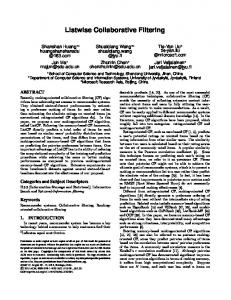
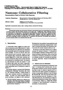
Figure 1: Item-based AutoRec model. We use plate notation to indicate that there are n copies of the neural network (one for each item), where W and V are tied across all copies. where h(r; θ) is the reconstruction of input r ∈ Rd , h(r; θ) = f (W · g(Vr + µ) + b) for activation functions f (·), g(·). Here, θ = {W, V, µ, b} for transformations W ∈ Rd×k , V ∈ Rk×d , and biases µ ∈ Rk , b ∈ Rd . This objective corresponds to an auto-associative neural network with a single, k-dimensional hidden layer. The parameters θ are learned using backpropagation. The item-based AutoRec model, shown in Figure 1, applies an autoencoder as per Equation 1 to the set of vectors {r(i) }n i=1 , with two important changes. First, we account for the fact that each r(i) is partially observed by only updating during backpropagation those weights that are associated with observed inputs, as is common in matrix factorisation and RBM approaches. Second, we regularise the learned parameters so as to prevent overfitting on the observed ratings. Formally, the objective function for the Item-based AutoRec (I-AutoRec) model is, for regularisation strength λ > 0, min θ
n X i=1
||r(i) − h(r(i) ; θ))||2O +
λ · (||W||2F + ||V||2F ), (2) 2
where || · ||2O means that we only consider the contribution of observed ratings. User-based AutoRec (U-AutoRec) is derived by working with {r(u) }m u=1 . In total, I-AutoRec requires the estimation of 2mk + m + k parameters. Given ˆ I-AutoRec’s predicted rating for user learned parameters θ, u and item i is ˆ u. ˆ ui = (h(r(i) ; θ)) R
(3)
Figure 1 illustrates the model, with shaded nodes corresponding to observed ratings, and solid connections corresponding to weights that are updated for the input r(i) .
U-RBM I-RBM U-AutoRec I-AutoRec
ML-1M 0.881 0.854 0.874 0.831
ML-10M 0.823 0.825 0.867 0.782
f (·) Identity Sigmoid Identity Sigmoid
(a)
g(·) Identity Identity Sigmoid Sigmoid
RMSE 0.872 0.852 0.831 0.836
BiasedMF I-RBM U-RBM LLORMA I-AutoRec
ML-1M 0.845 0.854 0.881 0.833 0.831
ML-10M 0.803 0.825 0.823 0.782 0.782
Netflix 0.844 0.845 0.834 0.823
(b)
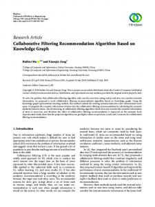
(c) Table 1: (a) Comparison of the RMSE of I/U-AutoRec and RBM models. (b) RMSE for I-AutoRec with choices of linear and nonlinear activation functions, Movielens 1M dataset. (c) Comparison of I-AutoRec with baselines on MovieLens and Netflix datasets. We remark that I-RBM did not converge after one week of training. LLORMA’s performance is taken from [2].
3.
EXPERIMENTAL EVALUATION
In this section, we evaluate and compare AutoRec with RBM-CF [4], Biased Matrix Factorisation [1] (BiasedMF), and Local Low-Rank Matrix Factorisation (LLORMA) [2] on the Movielens 1M, 10M and Netflix datasets. Following [2], we use a default rating of 3 for test users or items without training observations. We split the data into random 90%–10% train-test sets, and hold out 10% of the training set for hyperparamater tuning. We repeat this splitting procedure 5 times and report average RMSE. 95% confidence intervals on RMSE were ±0.003 or less in each experiment. For all baselines, we tuned the regularisation strength λ ∈ {0.001, 0.01, 0.1, 1, 100, 1000} and the appropriate latent dimension k ∈ {10, 20, 40, 80, 100, 200, 300, 400, 500}. A challenge training autoencoders is non-convexity of the objective. We found resilient propagation (RProp) [3] to give comparable performance to L-BFGS, while being much faster. Thus, we use RProp for all subsequent experiments: Which is better, item- or user-based autoencoding with RBMs or AutoRec? Table 1a shows item-based (I-) methods for RBM and AutoRec generally perform better; this is likely since the average number of ratings per item is much more than those per user; high variance in the number of user ratings leads to less reliable prediction for user-based methods. I-AutoRec outperforms all RBM variants. How does AutoRec performance vary with linear and nonlinear activation functions f (·), g(·)? Table 1b indicates that nonlinearity in the hidden layer (via g(·)) is critical for good performance of I-AutoRec, indicating its
0.87
0.86
RMSE
AutoRec is distinct to existing CF approaches. Compared to the RBM-based CF model (RBM-CF) [4], there are several differences. First, RBM-CF proposes a generative, probabilistic model based on restricted Boltzmann machines, while AutoRec is a discriminative model based on autoencoders. Second, RBM-CF estimates parameters by maximising log likelihood, while AutoRec directly minimises RMSE, the canonical performance in rating prediction tasks. Third, training RBM-CF requires the use of contrastive divergence, whereas training AutoRec requires the comparatively faster gradient-based backpropagation. Finally, RBM-CF is only applicable for discrete ratings, and estimates a separate set of parameters for each rating value. For r possible ratings, this implies nkr or (mkr) parameters for user- (item-) based RBM. AutoRec is agnostic to r and hence requires fewer parameters. Fewer parameters enables AutoRec to have less memory footprint and less prone to overfitting. Compared to matrix factorisation (MF) approaches, which embed both users and items into a shared latent space, the item-based AutoRec model only embeds items into latent space. Further, while MF learns a linear latent representation, AutoRec can learn a nonlinear latent representation through activation function g(·).
0.85
0.84
0.83
0.82
0
100
200 300 400 number of hidden units
500
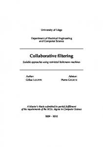
Figure 2: RMSE of I-AutoRec on Movielens 1M as the number of hidden units k varies. potential advantage over MF methods. Replacing sigmoids with Rectified Linear Units (ReLU) performed worse. All other AutoRec experiments use identity f (·) and sigmoid g(·) functions. How does performance of AutoRec vary with the number of hidden units? In Figure 2, we evaluate the performance of AutoRec model as the number of hidden units varies.We note that performance steadily increases with the number of hidden units, but with diminishing returns. All other AutoRec experiments use k = 500. How does AutoRec perform against all baselines? Table 1c shows that AutoRec consistently outperforms all baselines, except for comparable results with LLORMA on Movielens 10M. Competitive performance with LLORMA is of interest, as the latter involves weighting 50 different local matrix factorization models, whereas AutoRec only uses a single latent representation via a neural net autoencoder. Do deep extensions of AutoRec help? We developed a deep version of I-AutoRec with three hidden layers of (500, 250, 500) units, each with a sigmoid activation. We used greedy pretraining and then fine-tuned by gradient descent. On Movielens 1M, RMSE reduces from 0.831 to 0.827 indicating potential for further improvement via deep AutoRec. Acknowledgments NICTA is funded by the Australian Government as represented by the Dept. of Communications and the ARC through the ICT Centre of Excellence program. This research was supported in part by ARC DP140102185.
References [1] Y. Koren, R. Bell, and C. Volinsky. Matrix factorization techniques for recommender systems. Computer, 42, 2009. [2] J. Lee, S. Kim, G. Lebanon, and Y. Singer. Local low-rank matrix approximation. In ICML, 2013. [3] M. Riedmiller and H. Braun. A direct adaptive method for faster backpropagation learning: the rprop algorithm. In IEEE International Conference on Neural Networks, 1993. [4] R. Salakhutdinov, A. Mnih, and G. Hinton. Restricted Boltzmann machines for collaborative filtering. In ICML, 2007. [5] B. Sarwar, G. Karypis, J. Konstan, and J. Riedl. Item-based collaborative filtering recommendation algorithms. In WWW, 2001.