Hans-Peter Seidel. Hendrik P. A. Lensch. MPI Informatik. (a) Input images. (b) Computed labeling. (c) Estimated background. Figure 1: (a) Six photographs of the ...
Background Estimation from Non-Time Sequence Images Miguel Granados
Hans-Peter Seidel
Hendrik P. A. Lensch
MPI Informatik
(a) Input images
(b) Computed labeling
(c) Estimated background
Figure 1: (a) Six photographs of the Toscana scene featuring several transient objects. (b) For each background pixel the computed labeling selects the most consistent source image. (c) The estimated background image is free of temporal occluders. (bottom) Detail of a difficult region where the background is only visible in a single photograph.
A BSTRACT We address the problem of reconstructing the background of a scene from a set of photographs featuring several occluding objects. We assume that the photographs are obtained from the same viewpoint and under similar illumination conditions. Our approach is to define the background as a composite of the input photographs. Each possible composite is assigned a cost, and the resulting cost function is minimized. We penalize deviations from the following two model assumptions: background objects are stationary, and background objects are more likely to appear across the photographs. We approximate object stationariness using a motion boundary consistency term, and object likelihood using probability density estimates. The penalties are combined using an entropy-based weighting function. Furthermore, we constraint the solution space in order to avoid composites that cut through objects. The cost function is minimized using graph cuts, and the final result is composed using gradient domain fusion. We demonstrate the application of our method to the recovering of clean, unoccluded shots of crowded public places, as well as to the removal of ghosting artifacts in the reconstruction of high dynamic range images from multi-exposure sequences. Our contribution is the definition of an automatic method for consistent background estimation from multiple exposures featuring occluders, and its application to the problem of ghost removal in high dynamic range image reconstruction.
Keywords: background estimation, clean plate generation, energy minimization, graph cuts, HDR reconstruction, ghost removal Index Terms: I.4.8 [Image Processing and Computer Vision]: Scene Analysis: Time-varying imagery, color, depth cues— 1
I NTRODUCTION
Nowadays, digital photography consumer products are widely available, and photography enthusiasts and researchers are constantly exploring the possibilities beyond a single camera exposure. By taking multiple exposures using a tripod, and by processing them using standard image manipulation software, anyone can create novel images. Turning opaque objects into translucent, adding or removing transient objects, and compositing family portraits where everybody is smiling, are only few of the possible applications. In this paper, we focus on removing transient objects, i.e. to estimate the background of a scene, provided a set of exposures where the background is visible in at least some of them. Our aim is to perform this task in an automatic fashion. The input to our task is a set of low dynamic range color images (see Figure 1a). We assume all photographs are taken using the same viewpoint, camera configuration, and lighting conditions. These assumptions imply that if a scene object remains unaltered between two exposures, then the camera will register the same light rays. Our assumptions impose no restrictions on the time interval between exposures. The output is a low dynamic range color image featuring the scene background (see Figure 1c). The natural approach to the problem follows from the definition of background. Given an input set of images satisfying the aforementioned conditions, the background is the set of pixels repre-
senting objects whose distance to the camera is maximal. However, this definition implies the knowledge of pixel depth information. Although such information can be recovered using, for instance, stereo images or coded aperture [18], it is not available in our setup. Instead, we rely on the following model assumptions: background objects are more likely be photographed, and background objects are stationary. Our contribution consists of the assembling a model that defines the scene background as the minimizer of a cost function over composites of the input photographs. In particular, we derive a cost function by combining and extending ideas from Agarwala et al. [1] who addressed the problem of background estimation from still images by using a low likelihood penalty, and from Cohen [5] who performed background estimation from video sequences relying on a motion boundary inconsistency penalty. We increase the robustness of the background estimation by combining improved formulations of these two penalties using an entropy-based weighting function. Furthermore, we avoid partial classification of foreground objects as background by restricting the resulting composites to be locally consistent with at least one input photograph. While the derivation of our cost model, presented in Section 3, builds on the assumptions mentioned above, we further demonstrate the successful application of our pipeline on less restricted images, e.g. in the reconstruction of high dynamic range images from multiexposure series, discussed in Section 4.1. 2
R ELATED W ORK
Background estimation from time image sequences or videos has been extensively explored in the context of background removal, specially in motion tracking applications. Gordon et al. [10] exploit depth information recovered using stereo cameras in order to estimate and remove the background. In the case of image sequences where no depth information is available, several strategies have been applied: Kalman filtering [23], mixtures of Gaussians [26], non-parametric density estimation [8], mode estimation [20, 13], principal component analysis [19], optic flow [12], and energy minimization [5]. Following the latter strategy, Cohen [5] casts the problem of background estimation from videos as a labeling problem. His approach minimizes a cost function penalizing low color stationariness and motion boundary inconsistencies. Low color stationariness occurs at pixels with large temporal variance in a small time interval. Motion boundary inconsistencies occurs at pixels where the temporal gradient is large, i.e. the image starts to differ from others, but other images do not contain spatial gradient at that location (see Equation 4). In our work, we adapt this cost function to the case of non-time sequence images, by replacing the low color stationariness penalty with a term that does not require temporal coherence. Additionally, we adapt the motion boundary consistency penalty, and include an additional constraint for local consistency in order to ensure that the resulting background composite does not cut through objects. For non-time image sequences or photographs, background estimation has been previously approached using energy minimization [1], and mode estimation [2]. Agarwala et al. [1] apply energy minimization to a wide range of computer vision problems, background estimation among them, in a framework that allows assisted interactive retouch. For estimating the background, they define a cost function that includes a likelihood term penalizing pixel values with low probability. Per pixel probability distributions are estimated using histograms with fixed intervals. In our work, we include a more reliable likelihood term computed using non-parametric density estimators. This term, combined with a motion boundary consistency penalty, enables us to perform automatic background estimation (see Figures 5b and 5c).
Recently, Alexa [2] adapted the mean shift algorithm [6] to obtain robust estimates of the mode at every pixel location. In order to achieve spatial coherence, a metric which penalizes pixels differing from their neighbors is used. Spatial averaging is performed wherever a reliable estimation of the mode cannot be obtained. This unfortunately introduces blurring artifacts in the result (see Figure 5a) which our technique does resolve faithfully. A closely related problem to background estimation is the removal of ghosting artifacts in the reconstruction of high dynamic range (HDR) images from multi-exposure sequences [15, 16, 22, 14, 11]. For HDR video sequences, Kang et al. [15] apply motion compensation to align moving objects. For static scenes, since HDR images are typically computed as the weighted average of the linearized input images, it is relatively easy to decrease the influence of unreliable or fast moving objects. Pixels could be weighted based on its probability of belonging to the background [16], or single exposures could be selected to represent non-static scene regions [22, 14, 11]. While some of these techniques even provide registration techniques for hand held image sequences [27, 22, 11] we currently assume a static camera but could incorporate initial alignment. We apply our background estimation method to the reconstruction of HDR images from multi-exposure sequences (see Section 4.1). While previous approaches (with the exception of [16]) aim to reconstruct ghost-free HDR images, regardless of including transient objects in the final output, our method concentrates on reconstructing images featuring only the scene background.
3
BACKGROUND E STIMATION M ETHOD
3.1 Problem Statement We start by formally defining the problem’s input and output. Let I = {Il }N l=1 be an unordered set of input images. Let L = {1, . . . , N} be a set of labels, each corresponding to one image in I. Let Il (p) ∈ [0, 1]3 be the color value at pixel p of image l. Let P be the set of pixel positions p in any image. A labeling is a mapping f : P → L stating that a pixel p ∈ P has assigned the label f (p) ∈ L . We denote f (p) as f p for short. Every labeling f represents an image I f : p → I f p (p). Our task can be defined as obtaining a labeling f ∗ such that I f ∗ corresponds to the background image of I. The strategy for obtaining such a labeling is to assign a cost to each possible labeling, and then obtain the one with the minimum cost. Higher costs should be assigned to labelings as they deviate more from the model assumptions. Since range information is not available in order to distinguish foreground pixels, we construct a model based on the following assumptions: background objects are more likely to appear than transient ones, and background objects are stationary. The first assumption relies on the observation that most background objects are never occluded, and hence, the corresponding pixels should have high probability of occurrence. Therefore, we assign higher costs to labelings that choose pixels with low probabilities. The second model assumption restricts background objects to be static (flags or waving trees, for instance, do not fulfil it), and therefore, we penalize pixels indicating object motion. The resulting labeling might produce objectionable transitions between labeling regions (see Figures 6, 3b, 3c), introducing synthetic edges which have never been observed. Their influence can be reduced by enforcing the boundaries to occur in well-matching regions. Since the resulting transitions should be plausible with respect to our input data we also require the result to be locally consistent with at least one of the input images.
3.2 Energy Functional In order to represent the cost function, we define an energy functional of the form: E( f p ) =
∑ p∈P
Dp( f p) +
∑
Vp,q ( f p , fq ) +
(p,q)∈N
∑
H p,q ( f p , fq ),
(p,q)∈N
(1) where D p ( f p ) denotes the data term, and Vp,q ( f p , fq ), H p,q ( f p , fq ) denote the smoothness term and hard constraint, respectively. The data term defines the cost of assigning the label f p to pixel p. The smoothness term and hard constraint determine the cost of assigning the labels f p and fq to two neighbor pixels p, q. The set N denotes the set of 4-adjacent pixels in the image domain P. We describe each term in detail in the following sections. 3.2.1 Data Term The data term should indicate how well a pixel satisfies the model assumptions. Therefore, we include two parts in our data term: the Likelihood term DL , and the Stationariness term DS , each corresponding to one model assumption. The data term D at pixel p is defined as D p ( f p ) = (1 − β (p)) DLp ( f p ) + β (p)DSp ( f p ),
(2)
where β is a scalar that allows us to control the influence of each term. We will first introduce the likelihood and stationariness terms, and later discuss the choice for the β weights. Likelihood. Agarwala et al. [1] introduced a data term that penalizes pixel values which have low probability along the image set. At each pixel, they approximate the probability density function using histograms with fixed intervals. We benefit from smoother approximations using kernel density estimators. We define the likelihood penalty DL for a pixel p on the image f p as 3 Z I cf (p)+3λc p
DLp ( f p ) = 1 − ∏
c c=1 I f p (p)−3λc
dˆcp (x) dx,
(3)
where dˆcp is the estimated density function for the pixel p on the color channel c, and λc is the expected variation on each color channel. Note that the probability that a pixel value I f p (p) belongs to the background is computed as the joint probability over all color channels, assuming they are independent. For each channel c and pixel location p, we estimate the density function d cp (x) using Gaussian density estimators. The kernel bandwidths λc were obtained experimentally from datasets with known ground true. In Figure 2b, we illustrate the likelihood penalty assigned to one image from the Toscana scene. Note that the formulation of DLp requires that the probabilities on each color channel be independent. We satisfy this requirement by first transforming the input images to the Lαβ color space, which is known to be well decorrelated for natural images [21]. Stationariness. In order to approach our second model assumption, background stationariness, we incorporate the motion boundary consistency (MBC) term introduced by Cohen [5] in the context of background estimation from videos. In summary, the MBC term penalizes motion boundaries that do not occur at intensity edges of the background. Motion boundaries are approximated as the gradient of the difference between a photograph and the background. This is justified since the boundary of moving objects occur precisely at locations where the two images start to differ. Thus, assuming Ik is the background image and Il is an input photograph containing transient objects, motion boundaries are a subset of the edges of the difference image Ml,k = Il − Ik . The motion boundary inconsistency term validates that if Il displays the background at a given location, then large values of ∇Ml,k are also large in ∇Ik . In his formulation, Cohen defines every other input photograph
as background model, and averages their corresponding penalties, leading to the penalty
DSp ( f p ) =
1 N
∑ l∈L
2
∇M f p ,l (p) 2
k∇Il (p)k22 + ε 2
,
(4)
where ε is an arbitrary small value. Note that this formulation leads to arbitrary large penalties for k∇Il k2 approaching zero. However, in order to correctly balance the stationariness and the likelihood penalties, they are required to provide bounded responses. Therefore, we introduce a linear MBC approximation of the form (
∇M f (p) − k∇I(p)k ¯ ¯ if ∇M f p (p) 2 > k∇I(p)k S 2 2 p 2 Dp( f p) = 0 otherwise, (5) where M f p = I f p (p) − I¯ denotes the difference with the average image I¯ = N1 ∑l∈L Il , which is used as background model. The term response is restricted to the unit interval, provided that gradient magnitudes are normalized. Color gradient magnitudes are computed in the Di Zenzo [28] sense in the CIELAB color space. In Figure 2c, we present the stationariness cost corresponding to the second image from the Toscana scene (see Figure 1a). The benefits of the approximation of the background model as the average of the input exposures are twofold. First, the runtime complexity of the MBC term becomes linear in the number of images. Second, due to averaging, the intensity of true background edges is diminished by transient objects. This reduces the occurrence of false positive motion boundaries caused by flat, textureless occluders. Automatic Choice of β (p). The factor β (p) controls the relative importance of the stationariness and likelihood terms. Our aim is to select the appropriate factors in such a way that the most reliable information is preserved. We consider the set of observed intensities as a discrete random variable, and assign them probabilities proportionally to those already estimated in the likelihood term. The amount of information carried by this random variable can be measured by the entropy. This measure is maximized by uniformly distributed random variables, which do not carry information. We use this property and define the normalized entropy-based weight
β (p) = −
1 ∑ P p (l) ln(P p (l)), ln(N) l∈L
where P p (l) = 1 −
DLp (l) ∑k∈L DLp (k)
(6) (7)
is the normalized joint probability of exposure l at pixel p. The factor ln(N) maps the weights to the unit interval. In Figure 2d, we present the entropy image associated to the Toscana scene. High entropy values reduce the likelihood penalty influence. This can occur in two scenarios: the background is severely occluded, and the background is never occluded. In both cases, all photographs will have uniformly distributed probabilities (low and high respectively). In the case of an unoccluded background, this behavior is negligible since no likelihood penalty would be assigned. Interestingly, severely occluded regions also remain unpenalized. This enables the stationariness term in regions where likelihood information is scarce. Furthermore, whenever likelihood information is present, possible false positive motion boundaries are also down-weighted. In the remaining cases, i.e. when both terms are not reliable, we depend on the smoothness term to propagate information from neighboring pixels.
3.2.2 Smoothness Term
3.3 Parameters
In general, after minimizing the energy functional adjacent pixels are assigned to different labels. We would like such changes to occur in regions where two images match very well. To support this, we include a smoothness term that penalizes intensities differences along labeling discontinuities, as introduced by Kwatra et al. [17]. The smoothness term V is defined as
�
γ �
I f (p) − I f (p) + I f (q) − I f (q) . (8) Vp,q ( f p , fq ) = p q p q 2 2 2
The background estimation pipeline requires two input parameters: the smoothness weight γ , and the local consistency threshold tH . Both consider color discrepancies across labeling transitions. The local consistency constraint bounds the maximum color discrepancy across transitions. Discrepancies above the threshold tH are prohibited by assigning them an infinity cost. The selected threshold should account for the compounded noise of the capturing process, as well as for illumination variances. When the threshold is set too low, legitimate transitions between background regions are prevented. However, note that even for optimal threshold values visible artifacts still arise when illumination changes cause discrepancies below the threshold. In such cases, the algorithm would select any of the exposures under the threshold without regarding the closest match. This justifies the inclusion of a soft regularizer. The smoothness term weight γ controls the cost of introducing labeling discontinuities. The assigned cost depends linearly on the color discrepancy between the two incident images. As the smoothness parameter γ increases, the number of labeling transitions (and thus regions) decreases. The labeling energy also increases with the parameter γ , since there are less transitions available for moving to less costly areas. Nevertheless, since the maximum color discrepancy is bounded by the consistency constraint, the background can be correctly estimated for a wide range of γ values, provided that they are sufficiently small to allow enough labeling regions for compositing the background.
The penalty is only applied for f p 6= fq . Intensity differences are computed in a perceptually uniform color space, e.g. CIELAB. The γ factor controls the weight of the smoothness term. Higher γ values increase the cost of labeling discontinuities. This leads to fewer labeling regions. Note that the smoothness term is a soft regularizer, and its effect can be shadowed by large values in the data term. In order to ensure that the selected labeling discontinuities are plausible, we introduce a hard constraint that validates their consistency. 3.2.3 Hard Constraint for Local Consistency
We would like to ensure realistic background estimations, where transient objects are either completely included in or removed from the result. Including or removing whole objects would require accurate image segmentations, which are not always semantically consistent. Instead, we exploit the fact that the input images are intrinsically consistent by only allowing labeling discontinuities that result into transitions that have already been observed. This hard constraint for local consistency is defined as
( 0 if min I f p (p) − Il (p) + I fq (q) − Il (q) < tH l∈L H p,q ( f p , fq ) = ∞ otherwise. (9) The term H ∈ {0, ∞} assigns zero costs to consistent transitions and infinite otherwise. A transition is considered consistent if its color distance to the closest image l falls below a threshold tH . If the distance is too large, the transition is considered as never observed, and it is avoided by setting an infinite cost. In all our experiments we set tH to be 5% of the intensity range. The consistency term corresponds to a constraint on the solution space. It has been shown [25] that terms introducing zero or infinity costs satisfy the requirements of the expansion move algorithm (Section 3.4) for converging to strong local minima, as long as the initial solution has finite cost. Figure 6 exemplifies the effect of the constraint over a dataset where the background was not visible for all pixels.
3.4 Implementation The input images are first aligned in order to correct slight camera movements. We limit ourselves to translations with respect to a reference image, at sub-pixel resolution, choosing the translation with maximum cross correlation. The energy function E is minimized using the expansion move algorithm [4]. Briefly explained, given a label α ∈ L and a labeling f , an expansion is a labeling f ′ such that the energy of f ′ is strictly less than the energy of f , and the labelings only differ in a way that labels in f are replaced by α , i.e. assigning more pixels to the image α . Starting with an arbitrary labeling, the algorithm cycles through all labels, trying to find an expansion for each of them. Whenever an expansion is found, the current labeling is updated. The algorithm continues until a cycle over all labels does not decrease the energy any further. The key step in the algorithm is the expansion step, which is computed using graph cuts. For this step, we use the software library provided by Kolmogorov [3]. In a final stage, we perform gradient domain fusion [9] in order to correct any visible artifacts appearing due to illumination changes between photographs.
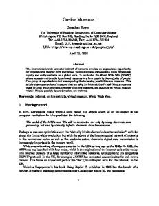
3.2.4 Interaction Between Terms The effect of each term in the energy functional is illustrated in Figure 3, which shows a detail of the Cathedral scene introduced by Agarwala et al. [1]. Figures 3b and 3c show the result obtained using only the likelihood and stationariness term, respectively. When omitting the smoothness term, the resulting labeling is locally optimized. Figure 3d shows the result obtained using the likelihood together with the smoothness term. Larger clusters appear since it is less costly to keep uniform labelings when transitions are not enforced by very unlikely regions. Observe that some transient objects persist in the result due their high probability. Figure 3e displays the result obtained using the stationariness and smoothness terms. The algorithm assigns a single label corresponding to an image featuring a blurred object with virtually no edge. The occluder goes undetected since it carries little gradient information. Lastly, Figure 3f shows the result obtained using the combined terms. The stationariness term rules out the occluders that the likelihood term alone could not detect, resulting in a more robust background estimation.
4
R ESULTS
For our experiments we generated two data sets named Toscana (6 images) and Market (12 images), presented in Figures 1 and 4, respectively. Both sets were captured using a tripod, and within a three minutes interval. The camera used was a consumer four megapixels Canon PowerShot A520, with minimum compression settings. The images were downscaled to a resolution of 1024x768 pixels. Each scene features both large and small scale transient objects, and natural lighting conditions. The resulting background estimation for the Toscana and Market sets are shown in Figures 1c and 4c, respectively. Each background computation took two minutes a standard desktop computer. The corresponding labelings are presented in Figures 1b and 4b. The smoothness term weight was set to γ = 12 and γ = 4, respectively, and the consistency threshold was set to 5% in both experiments. We further compare our method with the results reported by Agarwala et al. [1] and Alexa [2] (see Figure 5). For the comparison, we used a subset of 20 images from the Brandenburger Tor
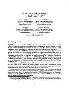
(a) Input
(b) DL
(c) DS
(d) β
(e) (1 − β )DL + β DS
Figure 2: Data term components: (a) Input image, (b) likelihood term DL , (c) entropy-based weights β , (d) stationariness term DS , (e) weighted sum. Red corresponds to values close to one, blue to values near zero.
(a) Input images
(b) DL
(c) DS
(d) DL +V
(e) DS +V
(f) (1 − β )DL + β DS +V
Figure 3: Interaction between the terms in the energy function. (a) Five photographs from the Cathedral scene [1]. (b) The likelihood term and (c) the stationariness term without regularization lead to locally optimized labelings. (d) The likelihood term alone fails to detect occluders in cluttered regions. (e) The stationariness term depends on gradient information and cannot detect flat or blurred objects. (f) The combination of both terms faithfully removes all occluders. In (b)-(f), the bottom row shows the computed minimum cost labeling, and the top row the corresponding background estimation.
(a) Input images
(b) Computed labeling
(c) Estimated background
Figure 4: (a) Eight (out of twelve) images from the Market scene. (b) Computed labeling. (c) Estimated background. The estimation removes all temporal occluders for which the background behind is visible. The hard constraint for local consistency constraint forbids partial removal of occluders. The sky region even though heavily segmented is smoothly reconstructed using gradient domain fusion.
scene introduced by Alexa [2]. The result by Alexa displays blurring artifacts, which are most evident under the gate (see Figure 5a); those artifacts are generated on regions where reliable mode estimations could not be obtained. In our approach, a single representative background image is selected and hence no blurring occurs. The result by Agarwala et al. (see Figure 5b) displays no blurring artifacts but still contains several transient objects at highly occluded background regions. In our method, due to the addition of the stationariness term, most transient objects are successfully removed. (see Figure 5c). Occluders remain in regions where the background was never visible, or whenever consistent transitions could not be included. 4.1 Application to High Dynamic Range Image Reconstruction As a final experiment, we apply our background estimation method to the problem of ghost removal in the reconstruction of high dynamic range images from multi-exposure sequences. For this experiment, we generated a dataset consisting of six photographs captured using exposure times 1/50s, 1/100s, 1/400s, 1/833s, and 1/1667. The dataset is presented in Figure 8a. We recovered the camera response function using the algorithm by Robertson et al. [24], and converted each photograph into relative radiance maps. It is critical that radiance values are consistent across exposures. For this reason, we adjust the exposure times in a way it minimizes the sum of squared intensity differences between consecutive exposures. The longest exposure is taken as starting point, and only correctly exposed pixels are accounted. We adapt our energy function in order to handle multi-exposure sequences. In the likelihood term, we need to exclude under- and over-exposed pixels from the probability density estimation. In the stationariness term, we also exclude such pixels from the averaged background model, since gradient information is likely to be lost. Furthermore, under- and over-exposed pixels are assigned an infinity cost in order to avoid their inclusion in the final labeling. Lastly, the constraint for local consistency is also made aware of such pixels, since consistency cannot be verified due to information loss. For this reason, only transitions occurring between well exposed pixels are validated. After the aforementioned modifications, the algorithm estimates an intermediate radiance map, where the value for each pixel is read from a single photograph. We use this result as a model for computing an averaged radiance map. The average only accounts for pixels whose difference with the intermediate model falls below a threshold. For tone mapping, we applied the adaptive logarithmic operator by Drago et al. [7]. Figures 8b and 8c show the resulting labeling and tone mapped background for the dataset. Note that the chrominance attributes of the tree and house front are visible simultaneously, which does not occur in any of the individual exposures. Furthermore, no ghosting artifacts appear from the transient objects in the scene. A reference image is presented in Figure 7 in order to illustrate the effect of considering an intermediate background model. 5
C ONCLUSIONS
We have presented an automatic algorithm for estimating a scene background from a set of non-time sequence photographs featuring several moving transient objects. The background is found by minimizing a novel cost function, which combines a measure for the likelihood of each input pixel being the background, with a motion boundary consistency term. The objective function is further weighted by an entropy measure that indicates how reliable the background likelihood is. We furthermore prevent the algorithm from cutting through objects by explicitly enforcing the output to be locally consistent with our input data. We minimize the cost function using the graph cut based expansion move algorithm, and
remove remaining gradient mismatches in the result using gradient domain fusion. We have demonstrated the suitability of our model on data sets with few image samples and severely occluded regions. We also compared our method with previous results by Agarwala et al. [1] and Alexa [2]. Our algorithm does not introduce blurring artifacts, avoids cutting through objects, and consistently removes more transient objects than previous approaches. We also demonstrate the application of our method to ghost removal in the reconstruction of high dynamic range images from multi-exposure sequences featuring multiple occluders. In the future we plan to investigate the application of the proposed error metrics to other sensor fusion tasks, e.g. 3D range scanning with temporal occluders. Acknowledgements We would like to thank Agarwala et al. [1] and Boykov and Kolmogorov [3] for making their source code publicly available. This work has been partially funded by a DFG Emmy Noether fellowship (Le 1341/1-1) and the Max Planck Center for Visual Computing and Communication (BMBF-FKZ01IMC01). R EFERENCES [1] A. Agarwala, M. Dontcheva, M. Agrawala, S. M. Drucker, A. Colburn, B. Curless, D. Salesin, and M. F. Cohen. Interactive digital photomontage. ACM Trans. Graph., 23(3):294–302, 2004. [2] M. Alexa. Extracting the essence from sets of images. In Proc. of the Eurographics Workshop on Computational Aesthetics, pages 113– 120, 2007. [3] Y. Boykov and V. Kolmogorov. An experimental comparison of mincut/max-flow algorithms for energy minimization in vision. IEEE Trans. Pattern Anal. Mach. Intell., 26(9):1124–1137, 2004. [4] Y. Boykov, O. Veksler, and R. Zabih. Fast approximate energy minimization via graph cuts. IEEE Trans. Pattern Anal. Mach. Intell., 23(11):1222–1239, 2001. [5] S. Cohen. Background estimation as a labeling problem. In Proc. of the 10th IEEE International Conference on Computer Vision (ICCV 2005), pages 1034–1041. IEEE Computer Society, 2005. [6] D. Comaniciu and P. Meer. Mean shift: A robust approach toward feature space analysis. IEEE Trans. Pattern Anal. Mach. Intell., 24(5):603–619, 2002. [7] F. Drago, K. Myszkowski, T. Annen, and N. Chiba. Adaptive logarithmic mapping for displaying high contrast scenes. Comput. Graph. Forum, 22(3):419–426, 2003. [8] A. M. Elgammal, D. Harwood, and L. S. Davis. Non-parametric model for background subtraction. In D. Vernon, editor, Proc. of the 6th European Conference on Computer Vision (ECCV 2000), volume 1843 of Lecture Notes in Computer Science, pages 751–767. Springer, 2000. [9] R. Fattal, D. Lischinski, and M. Werman. Gradient domain high dynamic range compression. ACM Trans. Graph., 21(3):249–256, 2002. [10] G. G. Gordon, T. Darrell, M. Harville, and J. Woodfill. Background estimation and removal based on range and color. In Proc. of the 1999 Conference on Computer Vision and Pattern Recognition (CVPR ’99), pages 2459–2464, 1999. [11] T. Grosch. Fast and Robust High Dynamic Range Image Generation with Camera and Object Movement. In Proc. of Vision Modeling and Visualization, pages 277–284, November 2006. [12] D. Gutchess, M. Trajkovic, E. Cohen-Solal, D. Lyons, and A. K. Jain. A background model initialization algorithm for video surveillance. In ICCV, pages 733–740, 2001. [13] B. Han, D. Comaniciu, and L. Davis. Sequential kernel density approximation through mode propagation: applications to background modeling. In Proc. of the Asian Conference on Computer Vision (ACCV 2004), 2004. [14] K. Jacobs, G. Ward, and C. Loscos. Automatic HDRI generation of dynamic environments. In Proc. of SIGGRAPH ’05: ACM SIGGRAPH 2005 Sketches, page 43, New York, NY, USA, 2005. ACM Press.
(a) Result by Alexa [2]
(b) Result by Agarwala et al. [1]
(c) Our result
Figure 5: Comparison with previous background estimation methods using 20 images (top, eight sown) from the Brandenburger Tor scene [2]. (a) The result by Alexa [2] features objectionable blurring artifacts. (b) The result by Agarwala et al. [1] features many remaining transient objects. (c) In our result, most transient objects are removed.
Figure 6: (left) Estimation obtained without the hard constraint for local consistency. (right) Result after including the constraint. In the input dataset, the background is not visible for all pixels.
(a) Sample input images
Figure 7: Ghost removal in HDR image reconstruction. (left) Due to averaging, transient objects appear as ghosting artifacts in the HDR image. (right) The estimated background model allows omitting the occluder’s contribution.
(b) Computed labeling
(c) Estimated radiance map (tone mapped)
Figure 8: Application of our method to ghost removal in high dynamic range image reconstruction. (a) Six input photographs captured with different exposure times (1/50s, 1/100s, 1/400s, 1/833s, and 2 × 1/1667s). (b) Color coded computed labeling. (c) Tone mapped background estimation. The result is a ghost-free high dynamic range image of the scene background.
[15] S. B. Kang, M. Uyttendaele, S. A. J. Winder, and R. Szeliski. High dynamic range video. ACM Trans. Graph., 22(3):319–325, 2003. [16] E. A. Khan, A. O. Aky¨uz, and E. Reinhard. Ghost removal in high dynamic range images. In Proc. of the International Conference on Image Processing (ICIP 2006), pages 2005–2008. IEEE, 2006. [17] V. Kwatra, A. Sch¨odl, I. A. Essa, G. Turk, and A. F. Bobick. Graphcut textures: image and video synthesis using graph cuts. ACM Trans. Graph., 22(3):277–286, 2003. [18] A. Levin, R. Fergus, F. Durand, and W. T. Freeman. Image and depth from a conventional camera with a coded aperture. ACM Trans. Graph., 26(3):70, 2007. [19] A. Monnet, A. Mittal, N. Paragios, and V. Ramesh. Background modeling and subtraction of dynamic scenes. In Proc. of the Ninth IEEE International Conference on Computer Vision (ICCV’03), page 1305, Washington, DC, USA, 2003. IEEE Computer Society. [20] M. Piccardi and T. Jan. Mean-shift background image modelling. In Proc. of the International Conference on Image Processing (ICIP 2004), pages 3399–3402, 2004. [21] E. Reinhard, M. Ashikhmin, B. Gooch, and P. Shirley. Color transfer between images. IEEE Computer Graphics and Applications, 21(5):34–41, 2001. [22] E. Reinhard, G. Ward, S. Pattanaik, and P. Debevec. High Dynamic Range Imaging: Acquisition, Display, and Image-Based Lighting (The Morgan Kaufmann Series in Computer Graphics). Morgan Kaufmann Publishers Inc., San Francisco, CA, USA, 2005. [23] C. Ridder, O. Munkelt, and H. Kirchner. Adaptive background estimation and foreground detection using Kalman filtering. In Proc. of the International Conference on Recent Advances in Mechatronics (ICRAM’95), pages 193–199, 1995. [24] M. A. Robertson, S. Borman, and R. L. Stevenson. Dynamic range improvement through multiple exposures. In Proc. of the International Conference on Image Processing (ICIP 1999), pages 159–163, 1999. [25] C. Rother, S. Kumar, V. Kolmogorov, and A. Blake. Digital tapestry. In Proc. of the 2005 IEEE Computer Society Conference on Computer Vision and Pattern Recognition (CVPR 2005), pages 589–596. IEEE Computer Society, 2005. [26] C. Stauffer and W. E. L. Grimson. Adaptive background mixture models for real-time tracking. In Proc. of the 1999 Conference on Computer Vision and Pattern Recognition (CVPR ’99), pages 2246–2252, 1999. [27] G. Ward. Fast, robust image registration for compositing high dynamic range photographs from hand-held exposures. Journal of Graphics Tools, 8(2):17–30, 2003. [28] S. D. Zenzo. A note on the gradient of a multi-image. Computer Vision, Graphics, and Image Processing, 33(1):116–125, 1986.