Balancing Closed and Open Loop CSI in. Mobile Satellite Link Adaptation. Alberto Rico-AlvariËno, Jesus Arnau and Carlos Mosquera. Signal Theory and ...
Balancing Closed and Open Loop CSI in Mobile Satellite Link Adaptation Alberto Rico-Alvari˜no, Jesus Arnau and Carlos Mosquera Signal Theory and Communications Department, University of Vigo, Galicia, Spain email: {alberto,suso,mosquera}@gts.uvigo.es
Abstract—We consider the problem of modulation and coding scheme selection in the return link of a mobile satellite system. We propose to use a weighted combination of both open loop and closed loop signal quality indicators to perform this selection. The combination weights are not selected by making any assumptions on the channel distribution; instead, they are dynamically adapted according to the ACK/NAK exchange between both ends. This adaptation procedure is obtained as a stochastic programming solution to an optimization problem. Numerical results will show the good performance of the proposed method compared to previous algorithms, and its robustness to environment changes. Index Terms—MCS selection, link adaptation, rate adaptation, mobile satellite, open loop, stochastic programming
I. I NTRODUCTION Link adaptation is the process of selecting an appropriate modulation and coding scheme (MCS) depending on the channel conditions. This adaptation is performed based on some sort of channel state information (CSI), such as signal to noise ratio (SNR), for example. This information has to be somehow acquired by the transmitter to select an MCS accordingly. There are two ways to acquire CSI, namely, open and closed loop (see Figure 1). Open loop CSI acquisition is based on channel reciprocity, i.e., the fact that channels in the uplink and downlink can be strongly correlated. This channel reciprocity can be also applied to the return and forward link in satellite communications. Closed loop CSI relies on a receiver estimating the channel response and feeding it back to a transmitter, usually by means of a limited feedback channel. Most modern two-way communication systems work in frequency division duplexing (FDD) mode instead of time division duplexing (TDD), and discard open loop operation due to the lack of channel reciprocity between different frequency bands. After the CSI acquisition stage, the transmitter selects an MCS for transmission. A typical approach is to assign MCS to SNR values by means of a look-up table (LUT), which has to be built by performing exhaustive simulations to determine Work supported by the Spanish Government under projects DYNACS (TEC2010-21245-C02- 02/TCM) and COMONSENS (CONSOLIDER INGENIO 2010 CSD2008-00010). Work supported by the European Regional Development Fund (ERDF) and the Galician Regional Government under agreement for funding the Atlantic Research Center for Information and Communication Technologies (AtlantTIC). Alberto Rico’s work was also supported by the Galician Regional Government Plan I2C under grant PRE/2013/469.
the performance of the different MCS, often assuming additive white gaussian noise (AWGN) conditions. This procedure is common in satellite communications, where hysteresis [1]–[3] is sometimes included. However, in practical scenarios the mapping between CSI and performance in AWGN may not be accurate: channels are time varying, receivers of different manufacturers may implement detection algorithms of different complexity, etc. To overcome this problem, backoff margins that depend on the statistical characterization of the channel have been introduced [1], [4]. These margins can be designed by following an LUTbased approach: again, exhaustive simulations are performed in many different scenarios, and the corresponding margins are calculated. These margins are stored in an LUT that is accessed by the transmitter to perform MCS selection. This implies that the simulations have to be representative of the scenarios where the communication system is going to operate, and that the transmitter is able to identify its environment. In consequence, this approach works only under controlled scenarios with calibrated receivers, and when the real-world parameters coincide with the simulated ones. Also, it requires the use of advanced algorithms to characterize the environment (e.g., speed, Rician K factor, line of sight (LOS) correlation, etc.). An alternative approach is to calculate this margin in an online manner, exploiting only the usual message exchange between transmitters and receivers. This approach, common in 3GPP systems [5], [6], has also been proposed for satellite communications [4], In general, the margins for open loop and closed loop CSI acquisition are different. A usual example arises in a natural way in the return link of satellite systems using FDD: open loop CSI is timely and inaccurate, whereas closed loop CSI is accurate but delayed [7], [8]. Previous work on open loop link adaptation for satellite calculated a margin by simulations [7] or derived it from a statistical characterization of the channel [8]. Also, it was identified that in some cases open loop works better than closed loop, even though a method to switch between both modes has not been proposed yet. In this paper, we propose an automatic mode switching and backoff margin calculator for link adaptation exploiting both open loop and closed loop CSI. We model the return and
Fig. 1.
Open-loop (left) against closed-loop (right) adaptation.
forward link as two channels with the same LOS components and uncorrelated non-LOS (NLOS). Both open loop and closed loop CSI are weighted depending only on the ACK/NAK exchange, as well as on the observed CSI. The backoff margin and CSI weights are derived as a stochastic programming solution to an optimization problem. The dynamic margin adaptation of [4] is obtained as a particular case of our method for fixed CSI weights. II. S YSTEM MODEL Consider a broadband global area network (BGAN)-like [9] mobile satellite link operating at the L-band; the forward link and return link frequency bands are centered at 1550 MHz and 1650 MHz, respectively1. In the following we describe the signal model in detail, along with some key system assumptions. A. Signal model Through this work we will assume that forward and return link channels experience the exact same LOS realization, but independent NLOS components with the same power and equal Doppler frequencies2. Focusing on the return link, whose signal parameters we seek to adapt, the signal model at a given time instant i is √ (1) yi = snr · hrl i si + wi
with yi the received symbol, si the transmitted symbol, hrl i the channel coefficient and snr the signal to noise ratio; accordingly, wi is the unit-power noise contribution. We now describe the channel model and present some assumptions on the coding of the system under study. Most of these characteristics will be used only for the evaluation of the proposed method, but not for its design. In fact, no particular probability density function (PDF) is assumed for the channel response, which has unknown parameters. Therefore, the proposed method is expected to be robust under channel modeling imperfections. 1 More precisely, the frequencies refer to the forward and return user links, or downlink and uplink of the user link. The feeder link, which is operating in a different frequency, is assumed to be transparent. 2 This is a simplification, as return and forward link operate in different frequencies. The difference between them, however, is less than 7%.
1) Channel model: For the simulations, we assume hrl i follows a Loo distribution [10]: slow variations in the LOS component (shadowing) are described by a log-normal distribution, whereas fast fluctuations of the signal amplitude (fading) are given by a Rician distribution. The PDF of the signal amplitude at a given time instant would be given by fr (x) = ∞
×
0
x √ b0 2πd0 1 x2 + z 2 (log z − µ)2 − exp − z 2d0 2b0
I0
x·z b0
dz (2)
where d0 and µ are the scale parameter and the location parameter of the log-normal distribution, respectively, and b0 is the variance of the Rician distribution; to determine these parameters we follow the Fontan 3-state model [11]. From an implementation point of view, the LOS component is generated in [11] by first obtaining independent and identically distributed (IID) Gaussian samples n, exponentiating them by 10(n/20) to obtain log-normally distributed numbers, and finally interpolating them to obtain the correlation properties specified by the model. This procedure, replicated in subsequent works on the topic, has two main drawbacks: the resulting sequence is not log-normal (interpolating a lognormal sequence does not preserve the original distribution), and the resulting process is not stationary but cyclostationary. Instead, we propose a procedure that preserves lognormality and ensures stationarity. Starting from i.i.d. Gaussian samples, the correlation properties are introduced before the exponentiation [7], [12] by a low pass filter whose cutoff frequency is given by fLOS = v · Tsymb /dc where v is the terminal speed, Tsymb is the symbol period and dc is the measured correlation distance of the LOS component, which we have obtained from [13]. We assume that the bandwidth of the system in both forward and return links is of 33.6 KHz, which leads to Tsymb = 1/(33.6 · 103 ) s. The NLOS component, on the other hand, is obtained by filtering complex Gaussian samples with a low-pass filter whose cutoff frequency is given by the Doppler spread.
+
channel with SNR γ and input restricted to a certain constellation {X1 , . . . , XL }
+
L
+
Θ (γ) = 1 − cL
+
ℓ=1
ǫi = Fig. 2. Diagram of the channel generation process, with xl ∈ {fl, rl}. α and Ψ are the location and scale parameters of the log-normal distribution.
To sum up, the forward and return link channels are generated by (see Figure 2 for a block diagram): (3)
2) Transmitted and received symbols: The transmitted symbols are the result of applying forward error correction coding and constellation mapping to a stream of bits; we consider a finite set of available codes, which are described in Table I. Symbols form codewords (4)
si = siN , siN +1 , . . . , s(i+1)N −1
of constant length N , such that they see the channel samples xl xl xl hxl i � hiN , hiN +1 , . . . , h(i+1)N −1
(5)
with xl ∈ {fl, rl}. For each sent codeword, we assume that the other end feeds back an ACK if decoding was possible, and a NAK otherwise. We assume that N = 2700, which gives codewords of approximately 80 ms. We neglect the effect of headers or other sort of overhead. B. Effective SNR Determining whether a codeword seeing different channel samples will be correctly decoded or not is a tough task. In general, the average SNR (possibly estimated from pilot symbols scattered through the codeword) is a poor indicator, as very different channel realizations could share the same value. To ease the simulation part, in this work, and as in [14], we will use an effective SNR metric instead, which is given by
xl � Θ−1 γeff,i
1 N
(i+1)N −1
k=iN
Θ snr · hxl k
2
.
e−
|Xℓ −Xk +w|2 −|w|2 1/γ
(7)
k=1
with cL = 1/(L log2 L) and w ∼ CN (0, 1/γ). Using this metric, we assume that the transmission of the ith codeword fails when γeff,i is below the threshold SNR of the MCS used, and that it succeeds otherwise. Define ǫi ∈ {0, 1} as the error event of the i-th codeword, then
+
LOS + hNLOS,rl , hfli = hLOS + hNLOS,fl . hrl i = hi i i i
L
E log2
(6)
This represents the SNR of an additive white Gaussian noise channel with the same mutual information as the faded channel hxl i , and with Θ (γ) the mutual information over a Gaussian
1 0
if γeff,i < γth otherwise.
(8)
The γth values in Table I are calculated as γth = Θ−1 (r), with r the spectral efficiency of each MCS. Note that, in this work, using the effective SNR is just a way of abstracting from the physical layer and reducing the simulation time; the design of the algorithm, its mathematical derivations and its performance do not rely on this assumption. III. P ROBLEM
STATEMENT
The objective of link adaptation is to select a proper MCS to maximize spectral efficiency with some constraint on the packet error rate (PER). Let us denote by mi ∈ {1, . . . , M } the index of the MCS selected in time instant i. We also assume that the error probability P [ǫi = 1] depends only on mi and hrl i , and thus is independent of the transmitted message. This assumption is compatible with the proposed error function (8), and holds for other error functions that characterize coded transmission. We denote the probability of error of the j-th MCS under channel hrl as E j, hrl , and assume that E j + 1, hrl ≥ E j, hrl , i.e., higher transmission rates imply higher error probabilities. The proposed adaptation method exploits both feedback from the receiver and SNR measurements in the forward link. We consider two types of feedback: first, the receiver acknowledges the correct decoding of the (i − d)-th codeword, so the values ǫ0 , . . . , ǫi−d are available at the transmitter at time instant i, with d the feedback delay; second, the receiver estimates the channel quality in time instant i − d and includes a channel quality indicator (CQI) in the feedback message. Although there are different ways to calculate the CQI, we consider the index of the highest MCS supported by channel rl ≤ pCQI . If no MCS hrl i , i.e., CQIi = arg maxj j|E j, hi is supported, then CQIi = 1. pCQI is a value that determines a limit on the error probability. In the case of using Gaussian coding with a sufficiently large code size, for example, pCQI can be set to a number as close to 0 as desired. With the proposed error function (8), the error probability can be set to zero if the channel is sufficiently favorable, so we assume pCQI = 0. The CQI value can be obtained from the effective SNR by means of a function Π. The function Π(SNR) is an LUT that maps SNR intervals to CQI values. Throughout the paper, we assume that the SNR values are in decibels for convenience. For M MCS values, the function Π can be
TABLE I C ODING RATE OPTIONS FOR THE R20T0.5Q-1B BEARER [9]. QPSK CONSTELLATION
Coding rate Rate (Spectral efficiency) γth (dB)
L8
L7
L6
L5
L4
L3
L2
L1
R
0.34 0.68 -2.1534
0.39 0.78 -1.3663
0.46 0.92 -0.3605
0.53 1.06 0.5733
0.61 1.22 1.5948
0.69 1.38 2.6092
0.73 1.46 3.1288
0.77 1.54 3.6674
0.81 1.62 4.2367
+ +
Fig. 3.
Diagram of the information exchange and link adaptation procedure.
parametrized by M − 1 thresholds tj , j = 1, . . . , M − 1, such that Π(SNR) = j ⇐⇒ tj−1 ≤ SNR < tj , where the higher and lower thresholds are defined as t0 = −∞ and tM = +∞. The function Π is usually referred to as inner loop for link adaptation, and we assume the thresholds to be the γth values for each MCS3 . If perfect SNR information was available at the transmitter, the link adaptation procedure would be trivial for a calibrated receiver. In practice, however, this information may not be available, so a correction has to be made to the estimated SNR value. We define ∐ as a function that maps MCS indexes to SNR values, such that Π (∐ (j)) = j. For example, a function that maps every MCS index to its SNR threshold γth meets this requirement, and is the one we will use throughout the paper. The objective of ∐ is to map CQI to SNR values. We also define SNRcl i � ∐ CQIi−d as the SNR that the transmit side gets to know about the received quality d frames earlier in closed loop mode. Note that SNRcl i denotes an estimate of the effective SNR performed in time instant i − d, but used at the terminal in instant i. In absence of feedback delay (d = 0), channel estimation error and other impairments, the optimal MCS selection would be mi = Π (∐ (CQIi )) = CQIi . A common practice to accommodate these impairments is the application of margins on the received CQI value, so cl mi = Π SNRcl i +c
(9)
with ccl the SNR margin in dB. A possible approach to select c is by means of an LUT that stores values of c for different 3 Note
that the γth for the first MCS is not used as a threshold.
scenarios, where parameters like channel distribution, Doppler, detection complexity, etc. have to be taken into account. This approach has some drawbacks that limit its application to practical settings. First, filling the LUT requires running exhaustive simulations under many different settings to be applicable to practical scenarios, and its behavior will be unpredictable under conditions that differ from the stored ones. Second, the receiver has to estimate the required parameters, which can be computationally expensive, and errors in the estimation of these parameters might lead to unexpected behavior. Thus, an adaptive method to adjust ccl is required in many cases. An adaptation of ccl based on ACK/NAK reception was proposed in [5], and applied to the satellite scenario in [4]. On top of the feedback information, the terminal is also observing the channel in the forward link. If the duplexing scheme was TDD, the terminal might gain access to timely and accurate CSI just by measuring the forward link channel. This sort of CSI is called open loop CSI. In our setting, duplexing is performed by means of frequency separation, so this assumption does not hold. Under our model, however, there is some degree of correlation between the forward and return link, as the LOS component is the same for both links. Therefore, depending on the scenario, the accuracy of the open loop CSI will vary. Let us define SNRol i as the most recent SNR estimation on the forward link. We assume that this SNR estimation is perfect, and equal to the effective SNR of the fl previous codeword, i.e., SNRol i = γeff,i−1 . This assumption does not affect the design of the method, and is made for the sole purpose of simplifying the simulations. We might think of performing a similar adaptation as in the closed loop case
(9)
A gradient descent iteration reads as mi = Π
SNRol i
+c
ol
(10)
.
Once again, the margin c should be obtained adaptively or by means of an LUT. In Figure 3 we show a diagram containing the main variables of the system model. A further question is how to determine the scenarios where (10) or (9) are more appropriate to be used. It is expected that in scenarios with relatively low speed or strong multipath the closed loop approach would perform better, while strong LOS and high speed scenarios are more suitable for the open loop one. As mentioned earlier, a possible approach is to perform parameter estimation (speed, multipath, etc.) and obtain the optimum strategy from an LUT, which had to be previously filled according to exhaustive simulation results. Alternatively, we present next an adaptive approach which avoids this cumbersome procedure and provides robustness by relying solely on the feedback of CQI and ACK/NAK, as well as on the open loop SNR estimation. ol
IV. A DAPTIVE CSI
BALANCING
A key observation in (9)-(10) is that they can be jointly described by cl cl mi = Π ξ ol SNRol i + ξ SNRi + c .
(11)
If we set ξ ol = 0, ξ cl = 1 we arrive to (9), and ξ cl = 0, ξ ol = 1 leads to (10). Note that (11) includes any affine combination of SNRol and SNRcl , so it generalizes the open loop and closed loop strategies. We now derive an adaptation method for general values of ξ cl and ξ ol , and in Section V we introduce a specific formulation if their sum is constrained to be one, ξ cl + ξ ol = 1. For simplicity, we denote SNRi �
ol SNRcl i SNRi
T
T
and ξ � ξ cl ξ ol ; the derivations from now on could be generalized for vectors SNR and ξ of any size, so we could include channel prediction in this framework, for example. Following a similar approach as [15], we state the problem of finding the margin c and SNR balancing weights ξ such that the packet error rate (PER) converges to a fixed target PER p0 . The desired values can be obtained as the solution to the following optimization problem min J(c, ξ) = |E [ǫ] − p0 |2 . c,ξ
(12)
Note that (12) does not have any optimality properties in terms of throughput, but just sets the mean packet error rate to the desired value p0 . In practice, nevertheless, it is expected that high SNR values will lead to the use of higher rate MCS to meet the target PER p0 , so the throughput is implicitly increased. Problem (12) can be solved by performing a gradient descent on J (c, ξ). The gradient of J(c, ξ) can be worked out as ∇J(c, ξ) = 2 (E [ǫ] − p0 ) ∇E [ǫ] .
(13)
ci+1 c = i − µi · ∇ J(c, ξ)|ci ,ξi . ξ i+1 ξi
(14)
Obtaining a numerical expression for the gradient J(c, ξ)|ci ,ξi is not possible: the expectation of ǫ depends on the PDF of the channel, which we assume unknown at the transmitter. On top of this, the PDF of the channel might change over time. Instead, we propose a stochastic gradient approach, where the expectations are substituted by instantaneous observations. Let us define (15) Ω � ξT SNR + c as the indicator SNR with which the MCS mi is selected in (11). Ω is a function of c and ξ whose gradient is trivial to compute, so that applying the chain rule of differentiation in (13) we arrive at ∇J(c, ξ) = 2 (E [ǫ] − p0 ) ∇E [ǫ] ∂ǫ ∇Ω = 2 (E [ǫ] − p0 ) E ∂Ω ∂ǫ 1 = 2E (E [ǫ] − p0 ) SNR ∂Ω
(16)
Following the stochastic gradient approach, we substitute E [ǫ] by the instantaneous value ǫi−d ; also, and since 2∂ǫ/∂Ω is positive4 , we embed 2E [∂ǫ/∂Ω] into the positive adaptation constant µi . The resulting expression for the update of c and ξ reads as (see Figure 4) ci+1 c 1 = i − µ (ǫi−d − p0 ) SNRi−d ξ i+1 ξi
(17)
where we have removed the dependence of µ with time, so we are using a constant stepsize. We shall notice that, in time instant i, the last received feedback is the one corresponding to the information transmitted in time i − d. The SNR values used for adaptation in (17) have to be the ones used for the MCS selection of the packet the ACK/NAK is referred to. Thus, if the transmitter knows the delay introduced by the channel, then a delay of z −d has to be introduced in the adaptation algorithm, as shown in Figure 4. On the other hand, if the delay value is not known or is variable (in case of ACK/NAK grouping, for example), then the transmitter should store the SNR values used for adaptation of every packet, indexed by a packet ID; when the ACK/NAK for a packet ID is received, the parameter update would be performed by recovering the corresponding SNR values from memory. Note that the closed loop SNR value SNRcl i used for MCS selection is the one generated by CQIi−d , but the one used for the adaptation of ξicl is SNRcl i−d , which is generated by CQIi−2d . 4 This can be proved by writing the probability of error, averaged over all channel states, in integral form, and using the assumption that for a channel state, the probability of error is higher for higher MCS. Higher values of Ω lead to higher MCS values, which increase the probability of error.
+
+
x
+
x
x
x
+
x
x
+
x
x
+
+
x
x
+
Fig. 5. Fig. 4.
Diagram of the adaptation process
Remark The adaptive margin algorithm proposed in [4], [5] is equivalent to the adaptation of c in (17). This adaptation is also the one described in [15]. More precisely, the algorithm for update described in [4], [5] is ci+1 =
if ǫi−d = 0 if ǫi−d = 1
ci + δup ci − δdown
(18)
with δup and δdown values such that5 δdown = δup
p0 . 1 − p0
(19)
It can be seen that (17) and (18) describe the same adaptation, provided that δup = µp0 and δdown = µ (1 − p0 ). V. C ONVERGENCE
ENHANCEMENTS
Simulations showed that the adaptation method described by (17) offers a noisy behavior in convergence, thus needing small values of µ which, in consequence, dramatically decreases the convergence speed. Note that (17) resembles a least mean T squares (LMS) adaptation with input [1 SNRi−d ] and error ǫi−d − p0 . Normalized LMS (NLMS) [16] is well known to outperform LMS in convergence speed. If the step-size is normalized in (17), the NLMS-like version reads as µ ci+1 c = i − ξ i+1 ξi 1 + SNRi−d
1 . SNRi−d (20) Note that we substituted p0 by p˜0,i . In general, (20) does not converge to a PER of p˜0,i , since the first component of a stationary point meets E
2
ǫi−d − p˜0,i
(ǫi−d − p˜0,i )
1 + SNRi−d
2
=0
(21)
5 In [4] the steps are selected to meet δ down = δup p0 instead of (19). Both formulations, however, are equivalent for low values of p0 .
+
x
+
+
x
+
Diagram of NLMS adaptation
which does not necessarily imply E [ǫi ] = p˜0,i . It is expected, however, that an appropriate choice of p˜0,i (not equal to p0 ) will lead to a PER of p0 . We propose to adjust p˜0,i following a recursion (22)
p˜0,i+1 = p˜0,i − λ (ǫi−d − p0 ) .
It is clear that E [ǫi ] = p0 is a stationary point of (22), thus leading to the desired PER. The desired value of p˜0 is expected to change very slowly, so a small value of λ should be selected. A block diagram of this NLMS adaptation is shown in Figure 5. It has been also observed that the NLMS adaptation offers a good convergence performance for the terms ξ, but not for the margin c, since the corrections to this term are smaller in absolute value than those for ξ because SNRol and SNRcl are usually larger than 1. To overcome this problem, we propose an alternative formulation that increases the speed of convergence of c µ ci+1 c = i − ξ i+1 ξi θ2 + SNRi−d
θ . SNRi−d (23) We also performed experiments with only one weight ξ instead of two. In this case, we defined the MCS selection rule as mi = Π
2
(ǫi−d − p˜0,i )
cl cl 1 − ξ cl SNRol i + ξ SNRi + c ,
(24)
and the corresponding adaptation rule as c ci+1 = cli − cl ξi ξi+1
µ ol θ2 + SNRcl i−d − SNRi−d
(ǫi−d − p˜0,i )
2×
θ . SNRcl − SNRol i−d i−d
(25)
and p˜0,i following the recursion in (22). The convergence properties of the methods described in this section are still being object of research. Nevertheless, their convergence to the desired PER value has been empirically observed, as described the next section.
0.18
Two ξ One ξ Open Loop Closed Loop
1.8 1.6
0.14 0.12
1.4 1.2 1
0.1 0.08 0.06
0.8
0.04
0.6 0.4
Two ξ One ξ Open Loop Closed Loop
0.16
PER
Spectral Efficiency (b/s/Hz)
2
0.02
0
1
2
3
4
5
6
7
8
9
0
10
0
1
2
3
LOS SNR (dB)
2
0.16
1.8
0.14
1.6
0.12
1.4
0.1
1.2 1
6
7
8
9
10
Two ξ One ξ Open Loop Closed Loop
0.08 0.06
Two ξ One ξ Open Loop Closed Loop
0.8 0.6 0.4
5
PER and throughput for different methods in intermediate tree shadowed environment, state 1, 0.3 m/s, p0 = 0.1
PER
Spectral Efficiency (b/s/Hz)
Fig. 6.
4
LOS SNR (dB)
0
1
2
3
4
5
6
7
8
9
0.04 0.02
10
LOS SNR (dB)
Fig. 7.
0
0
1
2
3
4
5
6
7
8
9
10
LOS SNR (dB)
PER and throughput for different methods in intermediate tree shadowed environment, state 1, 3 m/s, p0 = 0.01
VI. S IMULATION
RESULTS
We performed simulations of the proposed methods, given by equations (25) and (23), and compare them with open loop and closed loop with automatic margin adaptation, given by (18). The adaptation was performed with θ = 10, λ = 10−3 and µ = 1 for the case of the proposed methods, and µ = 10−2 for the open and closed loop cases, which correspond to δup = 0.001 and δdown = 0.009 for a target PER of 10−1 . The parameters were initialized as c0 = 0, ξ0cl = 0.5, and ξ0ol = 0.5. We set the feedback delay to d = 5 codewords to model the round trip time in a GEO satellite. Results were extracted for a Loo channel with the parameters of an intermediate tree shadowed environment, state 1 [11]; other settings were also tried, and similar results were observed. Three different terminal speeds were simulated: 0.3 m/s, 3 m/s and 15 m/s, with the corresponding target PER of 0.1, 0.01 and 0.1, respectively. Average spectral efficiency and throughput results were averaged over the transmission of N 6·104 packets. Spectral efficiency is defined as N1 i=1 ǫi rmi , with rj the rate of the j-th MCS. The obtained results are shown in Figures 6-8. It can be seen that the proposed methods fix the target PER more accurately than the others, and that in all cases the method with one ξ is more robust than the method with two ξ. Focusing on
the former, it always outperforms (or evens with) closed loop adaptation, and it also outperforms open loop adaptation in some cases. We shall remark that the target PER might not be achievable in very high or very low SNR scenarios. In these cases, the PER converges to the minimum or maximum possible PER values, respectively. VII. I MPLEMENTATION ASPECTS In this paper we made some simplifications to make the link adaptation problem more tractable. In the following, we comment on some possible implementation aspects of the proposed algorithm. a) CQI feedback: Throughout the paper, it was assumed that a CQI value was fed back for every packet. In modern communication standards this is not usually the case, so some packets would have a more outdated CQI than others. Assume that a CQI value is transmitted every K packets, then applying the same weight ξ cl in all K time instants could be suboptimal, since the first packet in every period has a much more precise CSI than the last one. A possible approach to overcome this problem is to have a different adaptation loop for each CQI delay. b) Use of effective SNR: Although in this paper we used effective SNR for convenience, the proposed method is
0.12
Two ξ One ξ Open Loop Closed Loop
1.8
1.6
0.1
Two ξ One ξ Open Loop Closed Loop
0.08
1.4
PER
Spectral Efficiency (b/s/Hz)
2
1.2
0.06
0.04 1 0.02
0.8
0
1
2
3
4
5
6
7
8
9
10
LOS SNR (dB)
Fig. 8.
0
0
1
2
3
4
5
6
7
8
9
10
LOS SNR (dB)
PER and throughput for different methods in intermediate tree shadowed environment, state 1, 15 m/s, p0 = 0.1
expected to work with other CSI metrics, such as average SNR or received signal strength indicator. This can be convenient in case the effective SNR calculation cannot be performed by the receiver. c) Interference in the return link: We neglected the possible interference in the return link, which is impossible to estimate from open loop observations [7]. In this case, the proposed method is expected to converge to weights ξ which account for the loss of reliability of the open loop CSI. d) Estimation errors and uncalibrated receivers: We assumed in the simulations that CQI and SNR estimates in the forward link were perfect, as well as the knowledge of the SNR thresholds for decoding. In practice, there might be some non-negligible errors in the SNR estimation, and the performance of a receiver might not be known a priori. In these cases, the proposed adaptive method is expected to adjust the parameters to meet the PER constraint, although possibly reducing the throughput with respect to the ideal case. e) Parameter divergence: In case of very high or very low SNR, the adaptation parameters ξ and c diverge, as it is not possible to converge to the desired PER p0 . A threshold should be included in the adaptation process to prevent this behavior. VIII. C ONCLUSION In this paper we presented a method for link adaptation in the return link of satellite communications that exploits open loop and closed loop CSI. The adaptive algorithm is obtained as a stochastic gradient descent of an unconstrained optimization problem. Interestingly, a baseline algorithm arises as a particular case of this optimization problem. The proposed method is shown to offer a good performance with respect to open loop and closed loop adaptation. R EFERENCES [1] S. Cioni, R. De Gaudenzi, and R. Rinaldo, “Adaptive coding and modulation for the forward link of broadband satellite networks,” in Proc. IEEE GLOBECOM, vol. 6, San Francisco, CA, Dec. 2003.
[2] ——, “Adaptive coding and modulation for the reverse link of broadband satellite networks,” in Proc. IEEE GLOBECOM, vol. 2, Dallas, TX., Nov. 2004, pp. 1101–1105. [3] ——, “Channel estimation and physical layer adaptation techniques for satellite networks exploiting adaptive coding and modulation,” International Journal of Satellite Communications and Networking, vol. 26, no. 2, pp. 157–188, 2008. [4] H. Bischl, H. Brandt, T. de Cola, R. De Gaudenzi, E. Eberlein, N. Girault, E. Alberty, S. Lipp, R. Rinaldo, B. Rislow, J. A. Skard, J. Tousch, and G. Ulbricht, “Adaptive coding and modulation for satellite broadband networks: From theory to practice,” International Journal of Satellite Communications and Networking, vol. 28, no. 2, pp. 59–111, 2010. [5] M. Nakamura, Y. Awad, and S. Vadgama, “Adaptive control of link adaptation for high speed downlink packet access (HSDPA) in W-CDMA,” in Proc. International Symposium on Wireless Personal Multimedia Communications, vol. 2, Oct. 2002, pp. 382–386 vol.2. [6] A. Muller and P. Frank, “Cooperative interference prediction for enhanced link adaptation in the 3GPP LTE uplink,” in Proc. IEEE VTC, Taipei, Taiwan, May 2010. [7] J. Arnau and C. Mosquera, “Open loop adaptive coding and modulation for mobile satellite return links,” in Proc. AIAA ICSSC, Firenze, Italy, Oct. 2013. [8] J. Arnau, A. Rico-Alvarino, and C. Mosquera, “Adaptive transmission techniques for mobile satellite links,” in Proc. AIAA ICSSC, Ottawa, Canada, Sep. 2012. [9] ETSI TS 102 744, “Satellite component of UMTS (S-UMTS); family SL satellite radio interface,” Oct. 2012, draft. [10] C. L. C. Loo, “A statistical model for a land mobile satellite link,” IEEE Trans. Veh. Technol., vol. 34, no. 3, pp. 122–127, Aug. 1985. [11] F. Fontan, M. Vazquez-Castro, C. Cabado, J. Garcia, and E. Kubista, “Statistical modeling of the LMS channel,” IEEE Trans. Veh. Technol., vol. 50, no. 6, pp. 1549–1567, Nov. 2001. [12] D. Arndt, T. Heyn, J. Konig, A. Ihlow, A. Heuberger, R. Prieto-Cerdeira, and E. Eberlein, “Extended two-state narrowband LMS propagation model for S-Band,” in IEEE Int. Symp. Broadband Multimed. Syst. Broadcast., Jun. 2012, pp. 1–6. [13] F. Perez-Fontan, M. Vazquez-Castro, S. Buonomo, J. Poiares-Baptista, and B. Arbesser-Rastburg, “S-band LMS propagation channel behaviour for different environments, degrees of shadowing and elevation angles,” IEEE Trans. Broadcast., vol. 44, no. 1, pp. 40–76, Mar. 1998. [14] K. Brueninghaus, D. Astely, T. Salzer, S. Visuri, A. Alexiou, S. Karger, and G.-A. Seraji, “Link performance models for system level simulations of broadband radio access systems,” in Proc. IEEE PIMRC, vol. 4, Berlin, Germany, Sep. 2005, pp. 2306–2311. [15] T. Cui, F. Lu, V. Sethuraman, A. Goteti, S. P. Rao, and P. Subrahmanya, “Throughput optimization in high speed downlink packet access (HSDPA),” IEEE Trans. Wireless Commun., vol. 10, no. 2, pp. 474–483, Feb. 2011. [16] S. Haykin, Adaptive filter theory. Prentice Hall, 2002.