University of Aleppo. Aleppo-Syria. AbstractâThis paper presents a newly developed approach for Differential Drive Mobile Robot (DDMR). The main goal is to.
(IJARAI) International Journal of Advanced Research in Artificial Intelligence, Vol. 4, No.5, 2015
A Novel Control-Navigation System-Based Adaptive Optimal Controller & EKF Localization of DDMR Dalia Kass Hanna, Bsc, Msc(Candidate)
Abdulkader Joukhadar, Bsc, MPhil, PhD
Mechatronics Department University of Aleppo Aleppo-Syria
Mechatronics Department University of Aleppo Aleppo-Syria
Abstract—This paper presents a newly developed approach for Differential Drive Mobile Robot (DDMR). The main goal is to provide a high dynamic system response in the joint space level, the low level control, as well as to enhance the DDMR localization. The proposed approach depends on a Linear Quadratic Regulator (LQR) for the low level control and an Adaptive LQR for the high level control. The investigated DDMR is considered highly nonlinear system due to uncertainty exhibited by the mobile robot incorporated with actuators nonlinearity. DDMR’s uncertainty leads to erroneous localization. An Extended Kalman Filter (EKF) -based approach with fusion sensors is used to enhance the robot degree of belief for its posture. Intensive simulation results obtained from the developed uncertain model and the proposed approach have shown very good dynamic performance on the low level control and very good convergence to the desired posture of the mobile robot path with the presence of robot uncertainty. Keywords—DDMR modelling; Localization; LQR; Adaptive LQR; EKF; System Uncertainty
I.
INTRODUCTION
The question of “where am I?” exhibited by mobile robots, in general, remains challenging and incompletely covered in academics. The topic of mobile robot localization has been paid wide attention by academics and industry to enhance the robot performance in different aspects for which the robot can perform its motion towards any desired posture with as minimum error as possible. Different techniques proposed to enhance trajectory tracking of wheeled mobile robots. [1, 2, 3, 4] utilize EKF algorithm with fusion sensors and gyroscope to localize the robot system as close as possible to the desired posture. The disadvantages of the work presented in [1, 2] do not pay attention to the dynamic performance of the system due to robot uncertainty but they considered only the noise affecting the proprioceptive and the exteroceptive sensors. However, in [2, 3] researchers use fusion sensors and vision sensor to help the system to be located correctly in a specific location. People in [3] implement EKF-based algorithm assisted with a gyroscope sensor to enhance the robot localization. Researchers in [3, 4] consider the proprioceptive sensors provide exact information about the robot motion in which the robot‟s posture is considered correct but noisy. Thus [3, 4] use EKF to purify the information about the robot‟s
localization. [6, 8] have proposed trajectory tracking algorithm but considered the information comes from the proprioceptive sensors is correct enough to determine the robot‟s posture with no lack of accuracy. The uncertainty of the mobile robot due to inaccuracy in the mechanical robot design and due to joint space inaccuracy exhibited by the mobile robot actuators lead to accumulated drift and divergence from the desired robot‟s posture. This paper focuses on a novel control approach utilizing Linear Quadratic Regulator for joint space control of robot actuators as well as proposing EKF-assisted optimal controller to overcome the problem of robot uncertainty, which may lead to robot posture divergence. The proposed approach is supported by fusion sensors consisted of a gyroscope sensor (rate & accelerometer) which is fixed to the robot‟s center of gravity and robot‟s on board sensors (odometry sensors). The onboard sensors (proprioceptive sensors) assumed noisy, in addition to the robot‟s mechanical parameters also considered highly uncertain. It is presumed, as well, that the mobile robot is due to some random disturbance represented by τd which is very common in the system control areas [3]. The remaining sections of the paper are as follows: Section II provides details about the dynamic model of the mobile robot incorporating the actuators dynamics; section III explains the design of the proposed controller for the joint space control system i.e., low level control; section IV discusses mobile robot navigation and localization; section V exhibits intensive simulation results with different system uncertainty and section VI provides a conclusion for the presented work. II.
DIFFERENTIAL DRIVE MOBILE ROBOT MODEL
A. Mobile Robot Motion Description: The HBE-RoboCar wheeled mobile Robot (WMR) has four driving wheels, which determine the moving direction of the robot through the rotating direction and speed of wheels. This WMR uses 4-DC geared motors for operation, and each wheel has one motor mounted. The wheels in the same side (left or right) are operated together as shown in Fig.1 to follow a certain robot trajectory. Such wheeled robots called Differential Drive Mobile robot (DDMR). In this section a mathematical description of DDMR moving on a planar surface is presented.
21 | P a g e www.ijarai.thesai.org
(IJARAI) International Journal of Advanced Research in Artificial Intelligence, Vol. 4, No.5, 2015
The study of DDMR motion is divided into three parts including kinematics, dynamics and drivers [8, 9]. B. Kinematic Model of the DDMR: Kinematics is the most basic study of how mechanical systems behave in order to model, analyze and simulate any control system design. The motion of this type of wheeled robot is classified as non-holonomic, which means, the motion constraint equations are needed to introduce into the DDMR‟s motion equations based on two main assumptions [9]:
Fig.1.
Block diagram of DDMR with actuators.
Usually, the DDMR‟s posture is determined in its environment based on two coordinate frames: the Global frame {G} and Local Frame {L}. The global frame is fixed in the environment in which the robot moves in. The local frame attached to the DDMR at the middle point A between two back wheels. The movement of point A represents the movement of the robot [9].
The robot can‟t move sideward. These non-holonomic constraints are taken into account by defining the velocity of the center point A in the local frame and forcing it to be zero. This constraint introduces in the global frame related to the velocity of point A by the following equation (1): x aG sin( ) y aG cos( ) 0
Where q G x aG the global frame.
y aG
T
(1)
is the coordinate of point A in
To simplify the model, it is assumed that each wheel has one contact point with the ground and there is no slippage in its longitudinal axis and lateral axis. The velocities of the contact points in the local frame are related to the wheel velocities by (2): VR rR
Fig.2.
(2) VL rL The linear and angular velocities of the DDMR related to the wheels velocities and the geometric parameters of the robot are given as follows (3):
DDMR Coordinates Systems
v (V R V L ) 2
As shown in Fig.2, x a and y a coordinate denote the position of DDMR in the global frame. The angle θ between the moving direction of the DDMR and the positive direction of the x-axis of the global coordinate frame denotes the orientation. Symbols used in this section are listed in Table1: TABLE I.
Description:
A
Distance between two wheels (m) The center of mass the middle point between two back wheels
d
Distance between A and C (m)
C
r
Wheel radius (m)
R , L
The angular velocity of the wheels (rad.s-1)
v ω N
The linear velocity of DDMR (m.s-1) The angular velocity of DDMR (rad.s-1)
Fig.3.
J
Gear ratio back emf constant ( vs.rad 1 ) Robot mass (kg) Robot moment of inertia (kg.m2)
FuR , FuL
Tangential forces exerted on DDMR by the wheels.
FwR , FwL
Radial forces exerted on DDMR by the wheels.
K M
(3)
KINEMATIC & DYNAMIC MODEL VARIABLES:
Parameter:
2L
(V R V L ) 2 L
The DDMR new position and orientation
To determine the new DDMR‟s position and orientation it is considered that the robot moves from the point A with a position ( x 1 , y 1 ), and orientation ( 1 NAC ) to A through a circular arc with an Instantaneous Center of Curvature (ICC) [2].
22 | P a g e www.ijarai.thesai.org
(IJARAI) International Journal of Advanced Research in Artificial Intelligence, Vol. 4, No.5, 2015
The increment of distance denoted by ( D ) and orientation denoted by ( ). As shown in Fig.3, based on triangular relationship the angle ( CAB 2 ) and the new orientation of DDMR given by (4):
1 2 (4) Considering that the increment of distance and orientation is small then AA D and the DDMR kinematic equation is given by (5): x x1 x q y y1 y 1 x1 D cos( 1 2) y1 D sin(1 2) 1 2
(5)
0 v 0 1
(8)
Mdv 2 L( R L ) r ( Md 2 J )
where FuR , FuL is linearly dependent on the wheel control input as follows: FuR R r , FuL L r Equations (8) represent the dynamic model of DDMR taking into account the non- holonomic constraints [9]. III.
Equation (5) is called Navigation Equation also. The navigation system analysis and design are based on equation (5). Another form for the kinematic model describes the robot behavior relative to the linear and angular velocities of the DDMR which can be written as follows (6): x GA cos G y A sin 0
Mv Md 2 2( R L ) r
CONTROLLER SYSTEM DESIGN:
In this section, a controller design based on solving quadratic optimal control problem has been presented to improve the dynamic performance of the DDMR for accurate trajectory tracking. Classical control methods are first designed and then their stability is examined. In optimal control, based on Liapunov approach the conditions for stability are formulated first and then the system is designed within these limitations. Thus, the designed system has a configuration with inherent stability characteristics [12].
(6)
The velocities of the center of mass C represented in the global inertial frame are given by (7): x CG cos G y C sin 0
d sin v d cos 1
(7)
Equation (7) is the relation between the velocities in local and global frames named as Guidance matrix G . C. Dynamic Model of the DDMR: In this subsection, the dynamic behavior of DDMR mechanisms based on Newton-Euler approach is presented [9]. By considering the free body diagram of DDMR; Fig.4 shows the forces acting on the DDMR [9].
Fig.5.
Optimal High and Low Level Control Structure Based DDMR.
The proposed control scheme shown in Fig.5 has two main controllers; high level control based on kinematic model of DDMR, that; correct the robot position and orientation to follow the commanded trajectory; and low level control based on dynamic model of DDMR which follows the velocities commands given by the high level controller. Both controllers employ quadratic optimal control approach. A. Low Level Controller: It is presumed in subsection (II, B) that, the linear and angular velocity of the DDMR related to the wheels velocities are given by (3) then the accelerations terms of the robot velocity and orientation angular speed are given by (9):
Fig.4.
v ( VR VL ) 2 w ( V V ) 2 L
Active Forces of the DDMR.
From Fig.4 the DDMR position, velocity and acceleration represented in the global frame using polar coordinate system and the equations (8) are divided using Newton‟s laws of motion in the robot frame:
R
(9)
L
By substituting (9) equations in the dynamic equation of DDMR (8):
23 | P a g e www.ijarai.thesai.org
(IJARAI) International Journal of Advanced Research in Artificial Intelligence, Vol. 4, No.5, 2015
VR 2 A R 2 B L 1 2 VL 2 B R 2 A L 1 2
(10)
Where 1 , 2 are the coupling terms between the left and the right wheels. An integral optimal control is proposed to control right and left wheels velocities by inserting an integrator in the feed forward path between the error comparator and the plant. Fig.6 shows the block diagram of the DDMR with optimal low level control.
seen the velocities of the center of mass C represented in the global frame are given by (7). It should be noted that the kinematic model of this type of wheeled robot is classified as nonlinear and involves nonholonomic constraints. To apply the optimal controller, a linear model of DDMR kinematic needs to be obtained. But if the linearization was about a stationary operating point the system become not controllable (In case that 0 and the DDMR move straightforward the information about y axes is lost. A novel technique is developed and applied on DDMR) by Adapting the discrete quadratic optimal algorithm to include this type of nonlinear systems using linear error model system along a desired trajectory [7]. First, equation (7) is discretized using the backward Euler method with sampling time Ts . The discretized form of DDMR kinematic model is obtained as shown in (14):
x k (v k cos k 1 dwk sin k 1 )Ts x k 1
(14)
y k (v k sin k 1 dwk cos k 1 )Ts y k 1
k wk Ts k 1 Fig.6.
or : x k f ( x k 1 , u k )
DDMR with optimal low level control.
The vector control u op which minimizes a selected cost function J given in (11) is determined as follow to solve the quadratic optimal control problem for the system given in (9): J
( x Qx u Ru )dt T
T
(11)
0
Where:
x41 : System state vector. u 21 : Vector control. Q44 : Positive semi-definite symmetric matrix determines the relative importance of the error. R22 : Positive definite symmetric matrix determines the relative importance of the expenditure of the energy of the control signals. The optimal control law is given as follows (12):
u op R
1
B1T
Px
(12)
P44 is the state covariance matrix which can be obtained from Reccati equation which is given as follows (13): (13) AT P PA PB1 R 1 B1T P Q 0 By designing the low level control system to have exponentially stable dynamic response with high dynamic performance response, the high level controller can be designed, considering linear dynamic response in the low level. B. High Level Controller: A proposed Adaptive Discrete Quadratic Optimal Controller formula based on DDMR kinematic system is described in this subsection. To derive the high level controller, the mathematical model of DDMR kinematic will be used. As
where xk xk
u k v k
k T is the system state vector and
yk
wk T is the input vector.
Second, defining the same equations for a desired trajectory generated by Guidance System as follows (15): xdk f ( xd k 1 , u d k 1 ) (15) The posture error vector e x k is given by (16):
e
e y k e k
xk
x T
dk
y d k d k T x k
y k k T
(16)
The velocities error vector eu k is given by (17):
ev k
ew k T v d k wd k T v k The linear error model is given by (18): e x k Fx e x k 1 Fu eu k
wk T
(17) (18)
Where: 1 0 (v d k sin( d k ) dwd k cos( d k ))Ts Fx 0 1 (v d k cos( d k ) dwd k sin( d k ))Ts 0 0 1 (19) Ts cos( d k ) dTs sin( d k ) Fu Ts sin( d k ) dTs cos( d k ) 0 Ts Fx , Fu are the Jacobian matrices of the system with respect to
e x k 1 , eu k respectively which was derived around a desired trajectory. Now, considering the following discrete cost function:
J
e
T k Qe k
u kT Ru k
(20)
0
The closed loop system state space will be (21):
24 | P a g e www.ijarai.thesai.org
(IJARAI) International Journal of Advanced Research in Artificial Intelligence, Vol. 4, No.5, 2015
e x k ( Fx Fu K )e x k 1 (21) Where K is the optimal control gain vector. These errors in position and orientation of DDMR are represented in the global frame, then the errors in the local frame have been found as follows (22):
eu k G 1e x k (22) The velocities commands which tracked by the low level control given by (23): v *R (v d k ev k ) L(wd k e w k )
(23)
v *L (v d k ev k ) L(wd k ew k )
IV.
NAVIGATION SYSTEM AND LOCALIZATION:
The robot navigation is the task of an autonomous robot to move safely from one location to another [13]. To make a truly autonomous robot an accurate localization is a key problem for successful navigation systems [4, 11]. The objective is to accurately determine DDMR‟s posture involving sensor noise uncertainties and potential failures in an optimal way with respect to a global or local frame of reference by integrating (fusing) kinetic information received from proprioceptive sensors (odometry and gyroscope) which give the robot feedback about its driving actions and obtaining knowledge about DDMR‟s environment [13]. In mobile robot navigation systems, onboard navigation sensors based on dead-reckoning are widely used. Dead reckoning is the process of calculating DDMR's current position by using a previously determined position and estimated speeds over the elapsed time [2, 5].
xk Ts cos( ) Ts cos( ) xk 1 y (1 2) T sin( ) T sin( ) VR k y k s s V k 1 L k Ts L Ts L k k 1
(24)
Second, note that equation (24) is nonlinear. So, in order to apply EKF algorithm, a linear approximation of Navigation Equation using Taylor series have to be obtained as follows (25):
xk J x xk 1 J u u k where:
x k x k u k [ VR k
yk
(25)
k
VL k ]
The terms J x , J u are the Jacobian which are obtained by differentiating equation (24) with respect to the state vector and input vector respectively (26): 1 0 vk Ts sin() J x 0 1 vk Ts cos( ) 1 0 0 vk vk Ts (cos( ) 2 L sin()) Ts (cos( ) 2 L sin()) v v J u (1 2) Ts (sin() k cos( )) Ts ((sin() k cos( )) 2L 2L Ts L Ts L
(26)
The EKF algorithm contains basically two main stages [10], Fig.7:
In the present section, EKF sensor fusion method is used for the estimation of DDMR‟s accurate posture and eliminates the effect of uncertainty associated with the system. The Extended Kalman filter (EKF) is a recursive optimum stochastic state estimator which can be used for parameter estimation of a non-linear dynamic system in real time by using noisy monitored signals that are disturbed by random noise [14, 15, 16]. The EKF has been widely used for mobile robot navigation and system integration to address the nonlinearity in the system kinematic. The goal of the EKF is to estimate the unmeasurable state (e.g. DDMR‟s posture) by using measured states, and also statistics of the noise and measurement (i.e. covariance matrices Q , R , P of the system noise vector, measurement noise vector, and system noise vector respectively) [15, 16, 17]. So the problem of mobile robot localization can usually not be sensed directly. The robot has to integrate data over time to determine its pose as accurate as possible using EKF fusion sensors method [4]. In order to apply the EKF algorithm [15], first, a discrete time Navigation Model for the DDMR based on equation (6) using the backward Euler method with sampling time Ts has been obtained (24):
Fig.7.
EKF Fusion Sensors Recursive Algorithm.
1) Action (or prediction) update: Having a priori knowledge implies that x k 1 , Pk 1 are initializing, the robot moves and estimates its position through its ideal proprioceptive sensors u k . (27) xˆ k f ( x k 1 , u k ) The covariance matrix after moving is given by (28): (28) Pk J x Pk 1 J xT J u QJ uT During this step, the robot uncertainty grows. 2) Perception (or measurements) update: The robot makes an observation using its uncertain model and corrects its position by opportunely combining its belief before the observation with the probability of making exactly
25 | P a g e www.ijarai.thesai.org
that observation. The Kalman gain is chosen to minimize the estimation error variance of the states to be estimated. (29)
The predicted state estimate ˆx k (and also its covariance matrix Pk ) is corrected recursively through a feedback correction scheme which is the product of the Kalman gain K and the deviation of the estimated measurement output vector and the actual output vector ( y ˆy ) that makes use of the actual measured quantities.
ˆx k ˆx k K k [ y k Hˆx k ] )Pk
Pk ( I K k H During this step, the DDMR uncertainty shrinks. If one looks at the problem of probabilistically, one can say that the robot has a degree of belief (bel) about where it is [5]. The goal of localization is to make this belief get as close as possible to the real distribution of the robot location. The robot incorporates these measurements into its belief to form a new belief about where it is [5]. The determinant of Pk provides a good measure of uncertainty as it is proportional to the volume of the deviation error ellipsoid. [5] The degree of belief is given by (31):
bel 1 det(Pk )
where 0 bel 1
(31)
The higher det( Pk ) is the less degree of belief there is in the measurements. V.
SIMULATION RESULTS:
The kinematics and dynamics model of the DDMR described in section II are used. The simulation is carried out by tracking different 3 DOFs desired paths with the high and low level control system of the DDMR. The proposed controlnavigation system is implemented based on the structures shown in Fig. 5. The DDMR with optimal low level control has been tested. Fig. 8.a shows the time response of the right and left motor wheels linear velocities and their corresponding control law i.e., actuator voltage control respectively to a step input command simulated using MATLAB/ Simulink. As seen from Fig. 8(a, b) the dynamic system response for the right and left wheels is high, and they converge to the desired set value exponentially with no overshot in the system response i.e., the equivalent damping ratio of the system is ζ=1. It is noted that the low level dynamic system is exponentially stable and shows high dynamic performance response with the limitation of 12volt
0.8 0.6 vR*[m/Sec] vR[m/Sec] vL*[m/Sec] vL[m/Sec]
0.4 0.2
0
2
4
6
8
10
Time [sec]
a.
Time Response for step commend 12 uR*[volt] uL*[volt]
10 8 6 4 2 0 -2
0
2
4
6
8
10
Time [sec]
b. Fig.8.
This section, several test results are demonstrated for the proposed control-navigation system based DDMR using MATLAB/ SIMULINK and C code.
1
0
(30)
The Control Voltage of Right and Left wheels[volt]
K k Pk H T [ HPk H T R] 1
Right and Left wheels Speed response[m/sec]
(IJARAI) International Journal of Advanced Research in Artificial Intelligence, Vol. 4, No.5, 2015
Motors voltages for left and right wheels Time responses of the right and left wheels velocity
Two experiments were performed and compared for DDMR with adaptive optimal high level control, with several trajectories to examine the robot dynamic performance, one was implemented utilizing only the onboard sensors data, and the other used EKF assisted fusion sensors method as navigation system considering different system uncertainty. A. Square Trajectory Tracking: This section demonstrates the mobile robot control performance to a square path with a side length of 1 meter. Fig. 9 shows the system dynamic response for the high-level control. As seen in Fig 9 that the system exhibited advancement trajectory tracking with a high degree of localization belief has explained by Fig. 10. As observed in Fig. 10 that the mobile robot system control in the high-level is very certain in its location i.e., where I am, since the degree of belief is high which is also very convincing indicator since the trajectory tracking error is negligible. Fig. 11 shows the mobile robot speed response, as seen in Fig. 11 the robot moved with maximum speed value 0.14 m.sec-1
26 | P a g e www.ijarai.thesai.org
(IJARAI) International Journal of Advanced Research in Artificial Intelligence, Vol. 4, No.5, 2015
The result, in this case, of Fig. 12, was obtained assuming the system is certain and there is no need to use any correction technique to correct the trajectory tracking.
1.5 ref path* [m] DDMR path [m]
Y trajctory [m]
1
It is seen that the system exhibited a very good convergence to the desired posture of DDMR. The same system is now tested presuming such uncertainty the robot model. It is to kindly remind the reader that the system is to work with no correction technique.
0.5
As seen in Fig. 13 the robot dynamics showed a remarkable divergence in the system trajectory tracking (see „black‟ reference trajectory and „blue‟ real trajectory).
0
-0.5 -0.5
0
0.5
1
Fig. 14 shows the robot‟s dynamic performance for an 8shape with presence of uncertainty in the mobile robot, but the control system was supported with a correction technique for posture correction („blue‟ is the reference trajectory, and „cyan‟ the real trajectory).
1.5
X trajctory [m]
Fig.9.
Square Trajectory EKF sensor fusion performance 1.2
5
ref path*[m] DDMR path [m]
degree of Belief
0.8 Y trajctory [m]
degree of Belief
1
0.6 0.4
0
0.2 0
0
10
20
30
40
50
60
-5
Time [sec]
Fig.10. The Degree of Belief for System Navigation
-5
0.15
5
Fig.12. DDMR Trajectory Tracking with Adaptive Optimal Control.
5
ref path*[m] DDMR path [m]
0.1 V[m/Sec] Y trajctory [m]
Mobile Robot Speed response[m/sec]
0 X trajctory [m]
0.05
0
0
5
10
15
20
25
0
30
Time [sec]
Fig.11. Speed Response of Mobile Robot
-5
B. Eight Shape Trajectory Tracking: This section provides two case simulation results for 8shape. These are simulation without system uncertainty and with system uncertainty. As seen in Fig. 12, the robot system tracks correctly the system the desired path (blue) and (red) real trajectory.
-5
0
5
X trajctory [m]
Fig.13. The Accumulated Divergence in the DDMR‟s Posture with Time
27 | P a g e www.ijarai.thesai.org
(IJARAI) International Journal of Advanced Research in Artificial Intelligence, Vol. 4, No.5, 2015
VI.
Y trajctory [m]
5
ref path*[m] DDMR path [m]
This paper has proposed a newly developed approach to enhance the dynamic response of a differential drive mobile robot with the presence of huge system uncertainty. The developed approach has considered a low-level system control developed on the joint space level (the actuators control level) and on the Cartesian space level control i.e., high-level control. For low-level control optimal type controllers (optimal and integral optimal) have been proposed for the actuator velocity control. It has been shown that the dynamic control response of the actuators is high and robust to system uncertainty.
0
-5 -5
0
5
X trajctory [m]
Fig.14. Path Correction based EKF Fusion Sensors Algorithm.
Fig. 15 shows that the proposed Control-Navigation system enhances the robot‟s belief at different points in time. The solid line displays the actions, and the ellipsoids represent the uncertainty effects on the robot‟s dynamic performance for the trajectory. DDMR path [m] uncertainty ellipsoid
-1.7
DDMR path [m] uncertainty ellipsoid
-1.8
0 uncertainty ellipsoid
uncertainty ellipsoid
5
-1.9 -2 -2.1 -2.2
In the high-level control, the system has been incorporated with Extended Kalman Filter (EKF) to estimate, as accurate as possible, the mobile robot posture. Simulation results obtained from the developed control system have shown that a large divergence was due to occur because of system uncertainty, which may lead to erroneous system localization as well as exhibited low degree of belief in the robot location. The proposed control approach in high-level domain overcomes the problem of robot‟s posture mismatch and tries to correct and compensate the trajectory tracking which may happen due to uncertainty. The interactive navigation process with the degree of belief, which reflects how the present robot‟s posture is close to the desired one. The validation of the proposed approach for lowlevel and high-level control has been confirmed through intensive simulation results obtained for different cases in which the robot has been imposed with uncertainty. As explained the proposed technique has given very encouraging results and has provided very good target tracking with high degree of belief for the robot localization. This work presented in this paper is basis for future. It is to be used for real time implementation for Mobile robot localization system control on the high and low levels identification e.g. UKF in real time utilizing dSPACE system board.
-2.3
-5
CONCLUSION
3
-2.4
-5
0
2.85
2.9
2.95
5
3
ref path*[m] DDMR path[m]
3.05
2
Time [sec]
Time [sec]
Fig.15. The Posture Believe‟s DDMR for 8 Shape.
C. Flower Shape Trajectory Tracking: More complex trajectory is used to examine the robot dynamic performance without the presence of uncertainty and with uncertainty. The system dynamic performance is shown in Figures 16, 17, 18 and 19. As noticed in Fig. 19 that the system showed high dynamic performance control for which is the system is capable to correctly track the desired path and even ensure high degree of belief for the robot posture. It can be observed that better performance control in real time has been obtained by integrating the control system (Low and high levels) with EKF fusion sensors approach to make the control system sensitive to the effects of the environment and able to eliminate the uncertainty effect.
Y trajctory[m]
1 0 -1 -2 -3 -3
-2
-1
0
1
2
3
X trajctory [m]
Fig.16. DDMR Trajectory Tracking with Adaptive Optimal Control
28 | P a g e www.ijarai.thesai.org
(IJARAI) International Journal of Advanced Research in Artificial Intelligence, Vol. 4, No.5, 2015
ACKNOWLEDGEMENT
3 ref path* [m] DDMR path [m]
2
The authors would like to thank the Syrian Society for Scientific Research (SSSR) for the financial support provided to cover SAI conference registration fee.
Y trajctory[m]
1
[1] 0 -1
[2]
-2 -3 -3
[3] -2
-1
0
1
2
3
X trajctory [m]
Fig.17. The accumulated divergence in the DDMR‟s posture with time.
[4]
3 2
Y trajctory [m]
[5]
ref path*[m] DDMR path [m]
[6]
1
[7]
0
[8] -1
[9] -2 -3 -3
-2
-1
0
1
2
3
[10]
X trajctory [m]
[11] Fig.18. Path Correction based EKF Fusion Sensors Algorithm. [12] [13] [14] [15] [16] [17]
REFERENCES Q. Meng, Y. Sun and Z. Cao “Adaptive Extended Kalman Filter (AEKF)-Based Mobile Robot Localization Using Sonar,” Robotica (2000), United Kingdom, Cambridge University Press, vol. 18, pp. 459473, ( December 1999). Y. Liu, Navigation and Control of Mobile Robot Using Sensor Fusion, Robot Vision, Ales Ude (Ed.), InTech, Available from: http://www.intechopen.com/books/robot-vision/navigationand-controlof-mobile-robot-using-sensor-fusion. (2010). S. Panich and N. Afzulpurkar “Mobile Robot Integrated with Gyroscope by using IKF,” International Journal of Advanced Robotic Systems, vol. 8, No. 2, pp. 122-136, (2011). R. Negenborn, “Robot Localization and Kalman Filters On Finding Your Position in a Noisy World”, UTRECHT UNIVERSITY (september 2003). S. Thrun, D. Fox and W. Burgard, “PROBABILISTIC ROBOTICS” Massachusttes Institute of Technology (2006). P. Jensfelt, “Approaches to Mobile Robot Localization in Indoor Environments”, Royal Institute of Technology (KTH), (2001). F. Kühne,W.F.Lages and Gomes da Silva Jr, “Model Predictive Control of a Mobile Robot using Linearization,”, IEEE Latin-American Robotics Symposium, pp. 525-530, ( 2005). K. Kozlowski and D. Pazderski, “Modeling and Control of a 4-wheel Skid- Steering Mobile Robot,”, Int. J. Appl. Math. Comput. Sci., vol. 14, pp. 477-496, ( 2004). R. Dhaouadi and A. Abu Hatab “Dynamic Modelling of DifferentialDrive Mobile Robots using Lgrange and Newton-Euler Methodologies: AUnified Framework,” Advance in Robotics & Automation, vol. 2, )Autom 2013(. S. Haykin, “Kalman Filtering and Neural Networks”, A WileyInterscience Publication, (2001). R. Siegwart and I. R. Nourbakhsh, “Introduction to Autonomous Mobile Robots”, The MIT Press,Cambridge, Massachusetts London, England, (2004). K. Ogata, “Designing Linear Control Systems With MATLAB”, Prentice Hall,(1994). P. Corke, “ Robotics, Vision and Control Fundamental Algorithms in MATLAB”, Springer Tracts in Advanced Robtics, vol 73, (2011). J.P. Norton, ”An Introduction to Identification”, Harcourt Brace Jovanovich, Publishers,(1986) P.S.Maybeck,”Stochastic models, estimation, and control”, Harcourt Brace Jovanovich, Publishers,(,vol 1, (1982) P.S.Maybeck,”Stochastic models, estimation, and control”, Harcourt Brace Jovanovich, Publishers,(,vol 2, (1982) P.S.Maybeck,”Stochastic models, estimation, and control”, Harcourt Brace Jovanovich, Publishers,(,vol 3, (1982)
Fig.19. The Posture Believe‟s DDMR for flower shape.
29 | P a g e www.ijarai.thesai.org