In Proceedings of the International Joint Conference on Neural Networks (IJCNN2000), Vol. II, pp. 113-117, July 2000.
The Inefficiency of Batch Training for Large Training Sets D. Randall Wilson
Tony R. Martinez
fonix corporation
[email protected]
Brigham Young University
[email protected]
Abstract. Multilayer perceptrons are often trained using error backpropagation (BP). BP training can be done in either a batch or continuous manner. Claims have frequently been made that batch training is faster and/or more "correct" than continuous training because it uses a better approximation of the true gradient for its weight updates. These claims are often supported by empirical evidence on very small data sets. These claims are untrue, however, for large training sets. This paper explains why batch training is much slower than continuous training for large training sets. Various levels of semi-batch training used on a 20,000-instance speech recognition task show a roughly linear increase in training time required with an increase in batch size.
1. Introduction Multilayer Perceptrons (MLPs) are often trained using error backpropagation (BP) (Bishop, 1995; Rumelhart & McClelland, 1986; Wasserman, 1993). MLPs consist of several layers of nodes, including an input layer, one or more hidden layers and an output layer. The activation of the input nodes are set by the environment, and the activation Aj of each node j in the hidden and output layers is set according to the equations: A j = f (S j ) =
1
1+ e S j = ∑ Wij Ai
−Sj
(1) (2)
i
where f() is a squashing function such as the sigmoid function shown, Sj is the weighted sum (i.e. the net value) of inputs from all nodes i on the previous layer, and Wij is the weight from node i (on the previous layer) to node j (on the current layer). The activation at the input layer is set by the environment. Once the activations of the hidden and output nodes are computed, the error is computed at the output layer and propagated back through the network. Weight changes for nodes are computed as: ∆Wij = r ⋅ Ai ⋅ δ j
(3)
where r is a global (often constant) learning rate, and δj is defined as (T j − A j ) ⋅ f ′ (S j ), if j is an output node; δ j = δ ⋅ W ⋅ f ′ (S ), otherwise. ∑ k jk j k
(4)
where i is again a node on the previous layer, k is a node on the following layer, Tj is the target value of an output node (e.g., 0 or 1), and f’() is the derivative of the squashing function f() with respect to the output activation. In continuous (often called on-line or sequential) training, the change in weights is applied after the presentation of each training instance. In batch training, the change in weights is accumulated over one epoch (i.e., over one presentation of all available training instances), and then weight changes are applied once at the end. Another alternative we call semi-batch, in which weight changes are accumulated over some number u of instances before actually updating the weights. Using an update frequency (or batch size) of u = 1 results in continuous training, while u = N results in batch training, where N is the number of instances in the training set.
2. Why batch training seems better When batch training is used, the accumulated weight change points in the direction of the true error gradient. This means that a (sufficiently small) step in that direction will reduce the error on the training set as a whole, unless a local minimum has already been reached. In contrast, each weight change made during continuous training will reduce the error for that particular instance, but can decrease or increase the error on the training set as a whole. For this reason, batch training is sometimes considered more "correct" than continuous training.
However, during continuous training the average weight change is in the direction of the true gradient. Just as a particle exhibiting Brownian motion appears to be moving randomly but in fact drifts in the direction of the current it is in, the weights during continuous training move in various directions but tend to move in the direction of the true gradient on average. Claims have also sometimes been made that batch training is "faster" than continuous training. In fact, the main advantage of continuous training is often cited as the savings in memory that come from not having to store accumulated weight changes. Speed comparisons between batch and continuous training are sometimes made by comparing the accuracy (or training error) of networks after a given number of weight updates. It is true that each step taken in batch training is likely to accomplish more than each step taken in continuous training, because the estimate of the gradient is more accurate. However, it takes N times as much computation to take a step in batch training as it does in continuous training. A more practical comparison is to compare the accuracy of networks after a certain number of training epochs, since an epoch of training takes approximately the same amount of time whether doing continuous or batch updates. However, empirical comparisons of batch and continuous training have usually been done on very small training sets. Hassoun (1995), for example, shows a graph in which convergence for batch and continuous training is almost exactly as fast on a sample application. However, as with many such studies, the training set used is very small— just 20 instances in this case. With such small training sets, the problems with batch training do not become apparent, but with larger training sets, it soon becomes obvious that batch training is impractical.
3. Why batch training is slower At a certain point in the weight space, a gradient can be computed expensively by batch training, in which case the gradient is accurate, or inexpensively by continuous training, in which case the gradient is questionable. No matter how accurate the gradient is calculated, however, it does not determine the location of the local minimum, nor even the direction of the local minimum. Rather, it points in the direction of steepest descent from the current point. Taking a small step in that direction will likely reveal that the direction at that new point is slightly different from the direction at the original point. In fact, the path to the minimum is likely to curve considerably, and not necessarily smoothly, in all but very simple problems. Therefore, though the gradient tells us which direction to go, it does not tell us how far we may safely go in that direction. Even if we knew the optimal size of a step to take in that direction (which we do not), we usually would not be at the local minimum. Instead, we would only be in a position to take a new step in a somewhat orthogonal direction, as is done in the conjugate gradient training method (Møller, 1993). Continuous training, on the other hand, takes many small steps in the average direction of the gradient. After a few training patterns have been presented to the network, the weights are in a different position in the weight space, and the gradient will likely be slightly different there. As training progresses, continuous training can follow the changing gradient around arbitrary curves and thus can often make more progress in the course of an epoch than any single step based on the original gradient could do in batch training. A small, constant (or slowly decaying) learning rate r (such as r = 0.01) is used to determine how large a step to take in the direction of the gradient. Thus, if the product δjAj from Equation (3) was in the range of ±1, then the change in weight would be in the range ±0.01, when doing continuous training. For batch training, on the other hand, such weight changes are accumulated N times before being applied. Suppose batch training is used on a large training set of 20,000 instances. Then weight changes in the same range as above will be accumulated over 20,000 steps, resulting in weight changes in the range ±200. Some of the weight changes are in different directions and thus cancel each other out, but changes can still easily be in the range ±100 (and in our experiments such magnitudes were not uncommon). Considering that weights are initialized to small random values smaller than ±1, this is much too large of a weight change to be reasonable. In order to do batch training without taking overly large steps, a much smaller learning rate must be used. Smaller learning rates require correspondingly more passes through the training data to achieve the same results. Thus, as the training set size grows, batch training gets correspondingly slower when compared to continuous training. If the size of the training set is doubled, the learning rate for batch training must be correspondingly divided in half, while continuous training can still be done with the same learning rate. Thus, the larger the training set gets, the slower batch training is relative to continuous training. With initial random (and thus poor) weight settings, together with a large training set, much of the initial error is brought down during the first epoch. In the limit, given sufficient data, learning would continue until some stopping criteria (e.g., a small enough total sum squared error or small validation set error), without ever having to do a second epoch through the training set. In this case continuous training would finish before batch training even did its first weight update. For our current example, batch training accumulates 20,000 weight changes based on random initial weights, leading to exaggerated overcorrection, unless a very small learning rate is used. Yet with a very small learning rate, the weights after 20,000 instances (1 epoch) are still close to the initial random settings.
Another approach we tried was to do continuous training for the first few epochs to get the weights in a reasonable range and follow this by batch training. Although this helps to some degree, empirical and analytical results show that this approach still requires a smaller learning rate and is thus much slower than continuous training, with no demonstrated gain in accuracy. Current research and theory is demonstrating that for complex problems, larger training sets are crucial to avoid overfitting and to attain higher generalization accuracy. Thus we propose that batch training is not a practical approach for future backpropagation learning approaches.
4. Empirical Results Experiments were run to see how update frequency (i.e., continuous, semi-batch and batch) and learning rates affect the speed with which neural networks can be trained, as well as the generalization accuracy they achieve. A continuous digit speech recognition task was used for these experiments. A neural network with 130 inputs, 200 hidden nodes, and 178 outputs was trained on a training set of N = 20,000 training instances. The output class of each instance corresponded to one of 178 context-dependent phoneme categories from the digit vocabulary. For each instance, one of the 178 outputs had a target of 1, and all other outputs had a target of 0. The targets of each instance were derived from hand-labeled phoneme representations of a set of training utterances. To measure the accuracy of the neural network, a hold-out set of multi-digit utterances was run through a speech recognition system. The system extracted Mel Frequency Cepstral Coefficient (MFCC) features from 8kHz telephone bandwidth audio samples in each utterance. The MFCC features from several neighboring 10 millisecond frames were fed into the trained neural network which in turn output a probability estimate for each of the 178 context-dependent phoneme categories on each of the frames. A decoder then searched the sequence of output vectors to find the most probable word sequence allowed by the vocabulary and grammar. In this case, the vocabulary consisted of the digits "oh" and "zero" through "nine," and the grammar allowed a continuous string of any number of digits. The sequence generated by the recognizer was compared with the true (target) sequence of digits. The number of insertions I, deletions D, substitutions S, and correct matches C, was summed over all utterances. The final word (digit) accuracy was computed as: Accuracy = 100% · (C - I) / T = 100% · (T - (S + I + D)) / T
(7)
where T is the total number of target words in all of the test utterances. Semi-batch training was done with update frequencies of u = 1 (i.e., continuous training), 10, 100, 1000, and 20,000 (i.e., batch training). Learning rates of r = 0.1, 0.01, 0.001, and 0.0001 were used with appropriate values of u in order to see how small the learning rate needed to be to allow each size of semi-batch training to learn properly. For each training run, the generalization word accuracy was measured after each training epoch so that the progress of the network could be plotted over time. Each training run used the same set of random initial weights (i.e., using the same random number seed), and the same random presentation order of the training instances for each epoch. When using the learning rate r = 0.1, u = 1 and u = 10 were roughly equivalent, but u = 100 did poorly. This learning rate was slightly too large even for continuous training and did not quite reach the same level of accuracy as smaller learning rates, while requiring almost as many epochs. When using the learning rate r = 0.01, u = 1 and u = 10 performed almost identically, achieving an accuracy of 96.31% after 27 epochs. Using u = 100 was close but not quite as good (95.76% after 46 epochs), and u = 1000 did poorly (i.e., it took over 1500 epochs to achieve its maximum accuracy of 95.02%). Batch training performed no better than random for over 100 epochs and never got above 17.2% accuracy. For r = 0.001, u = 1, and u = 100 performed almost identically, achieving 96.49% accuracy after about 400 epochs. Using u = 1000 caused a slight drop in accuracy, though it was close to the smaller values of u. Full batch training (i.e., u = 20,000) training did poorly, taking five times as long to reach a maximum accuracy of only 81.55%. Finally, using r = 0.0001, u = 1, u = 100, and u = 1000 all performed almost identically, achieving an accuracy of 96.31% after about 4000 epochs. Batch training remained at random levels of accuracy for 100 epochs before finally training up to an accuracy that was a little below the others. Using r = 0.0001 required over 100 times as many training epochs as using r = 0.01, without any significant improvement in accuracy. In fact, for batch training, the accuracy still was not as good as doing continuous training with r = 0.01. Unfortunately, realistic constraints on floating-point precision and CPU training time did not allow the use of smaller learning rates down to r = 0.01 / 20,000 = 0.0000005, which would have allowed a more direct comparison of continuous and batch training at the limit. (At that level we assume batch training would train as
well as continuous training, though requiring roughly 20,000 times as many training epochs as r = 0.01 with u = 1.) However, such results would contribute little to the overall conclusions of the practicality of batch training. Figure 1 shows the overall trend of the generalization accuracy of each of the above combinations as training progressed. Each series is identified by its values of u and r, e.g,. "1000-.01" means u = 1000 and r = 0.01. The horizontal axis shows the number of training epochs and uses a log scale to make the data easier to visualize. The actual data was sampled in order to space the points equally on the logarithmic scale, so caution should be used in using the individual peak points to surmise maximum generalization accuracy. Not all series were run for the same number of epochs, since it became clear that some had already reached their maximum accuracy before the 5000 epochs used by "1000-.0001". 1000-.0001
1-.001
97.00%
10-.01 1-.01
100-.001 100-.01
100-.0001 1-.0001
1000-.001
96.00%
1-.1
1-.1
10-.1
10-.1
95.00%
100-.1
1000-.01
Generalization Accuracy
94.00%
1-.01 10-.01
93.00%
100-.01
92.00%
1000-.01 20k-.01
91.00%
1-.001
20K-.0001
100-.001 1000-.001
90.00%
20k-.001 89.00%
1-.0001
88.00%
100-.0001 1000-.0001 20K-.0001
87.00% 1
10
100
1000
5000
Training Epochs
Figure 1. Generalization accuracy using various batch sizes (1-20,000) and learning rates (0.1-0.0001). Table 1 summarizes the maximum accuracy achieved by each combination of batch size u and learning rate r, as well as the number of training epochs required to achieve this maximum. Using a learning rate of r = 0.1 was slightly too large for this task. It required almost as many training epochs as using a learning rate that was 10 times smaller (i.e., r = 0.01), probably because it repeatedly overshot its target and had to do some amount of backtracking and/or oscillation before settling into a local minimum. Using learning rates of 0.001 and 0.0001 (i.e., 10 and 100 times smaller, respectively) required roughly 10 and 100 times as many epochs of training to achieve the same accuracy as using 0.01. Also, using learning rates of 0.01, 0.001, and 0.0001 allowed the safe use of semi-batch sizes of 10, 100, and 1000 instances, respectively, with reasonable but slightly less accurate generalization achieved by batch sizes of 100, 1000, and 20000, respectively. These results support the hypothesis that there is a nearly linear relationship between the learning rate and the number of epochs required for learning, and also between the learning rate and the number of weight changes that can be safely accumulated before applying them.
Therefore, for a large training set, using a Learning Batch Max Word Training semi-batch size of u requires roughly u times as Rate Size Accuracy Epochs Rating long to train when compared with continuous training. 0.1 1 95.76% 21 OK One potential advantage to batch training 0.1 10 95.94% 41 OK is that it allows parallel distributed training of a 0.1 100 92.99% 43 Bad single neural network. The N training 0.01 1 96.31% 27 Good instances can be broken up into M partitions of 0.01 10 96.31% 27 Good size N/M, where M is the number of machines 0.01 100 95.76% 46 OK available. Each machine can accumulate 0.01 1000 95.02% 1612 Poor weight changes for its partition, and then the 0.01 20,000 17.16% 381 Terrible weight changes can be accumulated, applied to 0.001 1 96.49% 402 Good the original weights, and rebroadcast to all the 0.001 100 96.49% 468 Good machines again. Ignoring weight accumulation 0.001 1000 96.13% 405 Good and broadcast overhead, each epoch would be 0.001 20,000 81.55% 1966 OK completed M times faster than training on one 0.0001 1 96.31% 4294 Good machine. Unfortunately, all M machines 0.0001 100 96.31% 4306 Good 0.0001 1000 96.31% 4282 Good would need to use a learning rate that is 0.0001 20,000 95.39% 3209 OK roughly N times smaller than that needed by a single machine doing continuous learning. This process is actually slower by a factor of Table 1. Overview of training time and accuracy for N /M than having a single machine doing various learning rates and batch sizes. continuous training with a larger learning rate. Using semi-batch training would suffer from the same problem and be slower by a factor of u/M.
5. Conclusions Batch training of multilayer perceptrons has occasionally been touted as being faster or more correct than continuous training, and has often been regarded as at least similar in training speed. However, on large training sets batch training must use a much smaller learning rate than continuous training, resulting in a linear slow-down compared to continuous training as training set size increases. While the gradient computed in batch training is more accurate than that used in continuous training, the average direction of the change in weights for continuous learning is in the direction of the true gradient. Furthermore, continuous training has the strong advantage of being able to follow curves in the error surface within each epoch, whereas batch training must take only a single step in one direction at the conclusion of each epoch. The results on a speech recognition task with 20,000 training instances lends support to the intuitive arguments in favor of using continuous learning on large training sets. Batch training appears to be impractical for large training sets. Future research will test this hypothesis further on a variety of neural network learning tasks of various sizes to help establish the generality of these conclusions.
References Bishop, Christopher M., (1995). Neural Networks for Pattern Recognition, New York, NY: Oxford University Press. Hassoun, Mohamad, (1995). Fundamentals of Artificial Neural Networks, MIT Press. Møller, Martin F., (1993). “A Scaled Conjugate Gradient Algorithm for Fast Supervised Learning,” Neural Networks, vol. 6, pp. 525-533. Rumelhart, D. E., and J. L. McClelland, (1986). Parallel Distributed Processing, MIT Press. Wasserman, Philip D., (1993). Advanced Methods in Neural Computing, New York, NY: Van Nostrand Reinhold.