Proceedings of the 6th Australian Joint Conference on Artificial Intelligence (AI’93), pp. 356-361, Nov. 1993.
The Potential of Prototype Styles of Generalization† D. Randall Wilson Tony R. Martinez Computer Science Department, Brigham Young University, Provo, Utah 84602 e-mail:
[email protected],
[email protected] Abstract. There are many ways for a learning system to generalize from training set data. This paper presents several generalization styles using prototypes in an attempt to provide accurate generalization on training set data for a wide variety of applications. These generalization styles are efficient in terms of time and space, and lend themselves well to massively parallel architectures. Empirical results of generalizing on several real-world applications are given, and these results indicate that the prototype styles of generalization presented have potential to provide accurate generalization for many applications. 1. Introduction There are many ways for a learning system to generalize from training set data. This paper proposes several generalization styles using prototypes in an attempt to provide accurate generalization on training set data for a wide variety of applications. These generalization styles are efficient in terms of time and space, and lend themselves well to massively parallel architectures. Traditional computer programming requires the programmer to explicitly define what the computer should do given any particular input. Even expert systems depend on the knowledge of experts in the field and their ability to explain how they make their decisions. When a solid knowledge of the application domain is available, this process has often worked quite well. In some applications, however, there is not enough known about the subject to derive a formula or write a program to solve the problem. In such cases, it is often possible to collect a set of examples of what the output of the system should be in specific situations. Each such example is called an instance, and usually consists of a vector of input values (the inputs) representing certain features of the environment, as well as the value(s) that the system should output in response to these input values (the output). A collection of such instances is called a training set. Neural networks1,2,3 provide one way to learn by example. That is, given a training set of instances, they can often “learn” the relationship between the inputs † This research was supported in part by grants from Novell, Inc., and WordPerfect Corporation.
Reference: The Sixth Australian Joint Conference on Artificial Intelligence (AI ’93), pp. 356-361, Nov. 1993.
and outputs well enough to be able to receive an input and produce the correct output with a high probability, even if that input did not appear in the training set. This ability is called generalization. Some styles of neural networks which have been successful in accurately learning to generalize from a training set, such as the backpropagation network4, have required many iterations through the learning algorithm to solve the problem, and thus have not always been able to solve problems in an acceptable amount of time. In addition, they often suffer from problems of getting stuck in a local minima, so several runs of the algorithm are often necessary. Some machine learning techniques attempt to generalize from training set data as well, but they often suffer from the problems of exponential search times and/or exponential storage requirements. The ASOCS (Adaptive Self-Organizing Concurrent System) model5,6,7 has the attractive feature of fast (one-shot) learning. It also lends itself to simple hierarchical architectures which can be efficiently implemented in hardware8. These features make it attractive for solving large problems very quickly, without hardware constraints. The ASOCS models, however, expect rule-based instances rather than training set data. In addition, some ASOCS models do not perform much generalization by themselves. The research presented in this paper began with the goal of extending ASOCS models to perform generalization on training set data. It makes use of several generalization styles in an attempt to provide accurate generalization which is efficient in terms of time and space, and which lends itself well to simple parallel architectures. In section 2, the styles of generalization studied in this research are presented, along with several extensions of each. Section 3 gives empirical results of simulations run on a variety of applications using each of these generalization styles, and gives a preliminary analysis of these results. Section 4 provides conclusions and future research areas. 2. Prototype Styles of Generalization The research presented in this paper makes use of several generalization styles which use prototypes in an attempt to provide accurate generalization in an efficient and potentially parallel manner. Prototypes are similar to instances in the training set, but may represent several instances with the same output, and can have additional features. When prototypes are used, they are compared with new inputs to determine the output. In such approaches, generalization styles determine both how the prototypes are created and how they are used. In this research prototypes consist of:
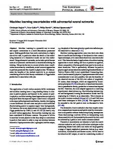
• A vector of input values representing features in the environment (inputs) and one or more output values, representing the supposedly correct response of the system to the input values (output). • A count of how many instances the prototype represents, • A count of how many instances with the same inputs had different outputs ( the conflict), • A ratio of count to total, where total = count + conflict. This gives a probability that the inputs of the prototype should map to its output(s), and is called the integrity. Figure 1, below, illustrates an typical instance in a training set and a prototype. Instance Inputs Output A BC D Z
Prototype Inputs Output A BC D Z Occurances + Integrity +/∑ Conflict –
Figure 1. Instance vs. Prototype
The styles of generalization presented in this paper have several attractive features: • They can learn a training set quickly (usually in O(n) or O(nlogn) time), • They are simple and intuitive, • They lend themselves well to massively parallel architectures (e.g. a binary tree) • They do not suffer from exponential storage or processing problems. On the other hand, they do store most of the instances in the training set, which can be sizable for large training sets, and because they do not throw away any information, they may “overlearn” the training set instead of picking out only the most relevant attributes of an application. This can result in a susceptibility to noise and reduced generalization. Several styles of generalization were used in this research, among which were several distance metrics, and some critical variable detection algorithms, along with voting schemes to enhance each of these. These styles are discussed in sections 2.1 and 2.2 below. 2.1. Distance Metrics Distance metrics are used to find out which prototype or prototypes are “closest” to the new input in question. The output value of the closest prototype or group of prototypes is used for the output value in response to the new input. There are several ways of determining how “close” an input is to one of the
prototypes. Hamming distance. Hamming distance is an intuitive metric, and is simply the number of input variables which do not match the prototype. The prototype with the least number of mismatched variables wins using this metric. State difference. In multi-state variables where the states represent a linear value, the closeness of the state number itself may help indicate the “distance” of an input variable to a variable in an instance. Thus, a sum of the (absolute) differences of the inputs of the prototype from the inputs of the new input can be used as a measure of closeness. Dividing by number of states. An extension of the State Distance scheme is to divide the state difference for each variable by the number of states that that variable can have, in order to normalize the distance measures. This can be done for Hamming distance as well. Euclidean distance. Euclidean distance is similar to the State Difference scheme, except that the individual distances are squared before they are summed. As an example, consider a training set with four input variables, the first three of which are Boolean, and the last of which is a 10-state variable (with values 0 through 9). If a prototype with input values 0, 0, 1, and 5, respectively, was compared to the input 0, 1, 1, 1, the distance metrics mentioned above would be computed as shown in Figure 2.
Variable Name: Number of States: Prototype: New input to be classified:
A 2 0 0
B 2 0 1
C 2 1 1
D Out 10 2 5 -> 1 1 -> ?
Distance Metric 1. Hamming Distance: 2. Hamming/No. of States: 3. State Difference: 4. State Diff/Num States: 5. Euclidean Distance:
Distance 0+1 +0+1 =2 0 + 1/2 + 0 + 1/10 = 0.6 0+1 +0+4 =5 0 + 1/2 + 0 + 4/10 = 0.9 0 + 1 + 0 + 16 = 17
Figure 2. Results of various distance metrics (from example 1).
Voting. Regardless of the distance metric used, there will often be several prototypes which are the same “distance” from the new input. Instead of arbitrarily choosing one of the several equally close prototypes to be the winner, the prototypes can vote for their output. One way to do this is to let each of these prototypes cast a number of votes equal to its count, since prototypes may represent several instances. 2.2. Critical Features. One way to determine which variables are most important is to find those which tend to have a strong correlation with an output value. In order to discover critical variables, a new kind of prototype called a first-order feature is created for each input variable of each instance. Each feature has only the output and one input variable asserted, and the rest of the input variables are “don’t
care” variables (denoted by an asterisk, “*”). It is possible to use combinations of variables instead of only one variable at a time and thus create higher-order features, but such methods run into exponential factors in both storage and computation time, and are thus not pursued in this research. The term feature will therefore be used to mean first-order feature. As an example, the instance “0 0 1 5 -> 1”, would result in the following four first-order features: “0***->1”, “*0**->1”, “**1*->1”, and “***5->1”. If any of these features already existed in the system, the new one would be discarded, and the old one’s count would be incremented and its integrity recomputed. If any features existed which had the same input but a different output (e.g., 0 * * * -> 0), then both features would increment their conflict and recompute their integrity. The first few instances in the training set will probably add quite a few features to the system, but later instances will usually find matches for most of the features they try to add. During generalization, a feature is said to match the input if the variable which is asserted matches the corresponding variable in the input. The other “don’t care” variables are always considered to match. In Figure 3, a few instances from a training set are listed, along with the features that would be generated for the first and second variables. Note that the conflict field is simply the sum of the counts of all other prototypes with the same inputs. Instances A B C D -> Out 0 1 1 3 0 0 0 0 0 1 0 0 1 0 1 0 1 1 5 1 1 1 0 1 0 1 0 1 0 1 • • •
First-order Features A B C D -> Out Frequency Conflict Integrity 0* * * 0 1 3 1/4=.25 0* * * 1 3 1 3/4=.75 1* * * 0 1 1 1/2=.50 1* * * 1 1 1 1/2=.50 *0 * * 1 3 0 3/3=1.0 *1 * * 0 2 1 2/3=.66 *1 * * 1 1 3 1/3=.33 • • •
Figure 3. Features generated from instances.
There are several ways to use these prototypes for generalization. One is to select the one very best feature that matches the input and use its output. The “best” feature can be either the one with the highest count (meaning it occurred most often), or the one with the highest integrity (meaning it was relatively undisputed). Another method is to select the best feature for each input variable, and let these vote on the output. A third method is to allow all matching features to vote for the output they want. In each case, a feature’s voting power equals its count, which is the number of instances it represents.
A 1. 0 2. 0 3. * 4. * 5. * 6. * 7. *
BCD * * * * * * 1 * * 1 * * * 1 * * 1 * * * 1
-> Out Count -> 0 1 -> 1 3 -> 0 2 -> 1 1 -> 0 1 -> 1 3 -> 0 1
Conflict 3 1 1 2 3 1 0
Integrity .25 .75 .66 .33 .25 .75 1.0
Figure 4 Features matching an input of “0 1 1 1”.
To continue the above example, assume that the rest of the features for the instances listed in Figure 3 were available. Given an input of 0 1 1 1, the features shown in Figure 4 would match the input. The one with the highest integrity is feature 7, which was never contradicted, and it would choose an output of 1. The one with the best count is either #2 or #6, both of which also opt for an output of 1. The features in bold (numbers 2, 3, 6 and 7) are the best in terms of both integrity and count for the four input variables, respectively. These would cast 2+1=3 votes for an output of 0, and 3+3=6 votes for an output of 1, so 1 would win again in this case. Finally, if all of these matching features were allowed to vote, an output of 0 would get 1+2+1+1=5 votes, and an output of 1 would get 3+1+3=7 votes. In this example, all of the various styles chose an output of 1, but there are cases in which the styles would pick conflicting outputs. 3. Empirical Results Each of the generalization styles described above was implemented and tested on several well-known training sets from the repository of Machine Learning Databases at University of California Irvine9, and the generalization accuracy of each style on each application is given in Table 5. The column labeled “Max” contains the maximum generalization accuracy of any of the styles for each application. The applications are ordered from best to worst in terms of maximum generalization ability. The results are encouraging, for they suggest that prototype styles of generalization can be effective on many applications, although there were some applications for which none of the styles was able to achieve acceptable generalization. There are a few interesting things to note from this table. First of all, note that there was no one style which generalized most accurately on all applications. This suggests that by using a collection of simple generalization styles, and by picking the one that did the best on the test set, the best style for a given
Max
application can be found 10 . Also note that the distance metric styles of generalization that used voting did as well or better than their corresponding nonvoting style in almost every case. First-Order Features Hamming State Euclid Single Best All Distance Distance ones vote best . Dist. one vote /#st. /#st. 1st vt 1st vt 1st vt 1st vt 1st vt cnt int cnt int cnt int
l00 99 98 96 95 93 93 88 87 86 81 77 76 72 70 53
l00 98 89 91 89 93 91 84 87 81 75 63 73 64 58 38
Distance Metrics
Database Soybean (Small) Zoo Vowel Iris Segmentation House-Votes-84 Soybean (Large) Sonar Shuttle-Landing Credit-Screening Audiology Nettalk Glass Indians-Diabetes Hepatitis Lung-Cancer
l00 97 91 90 90 93 93 84 87 81 77 77 74 65 59 34
l00 98 89 91 89 93 90 84 40 81 78 63 73 64 61 38
l00 97 91 90 90 93 91 84 40 81 81 77 74 65 59 34
l00 l00 99 98 97 97 96 95 94 95 93 93 89 87 88 87 87 87 76 76 68 71 48 59 74 76 67 66 59 60 41 47
l00 98 97 96 94 93 92 87 53 82 78 48 73 67 63 41
l00 98 97 95 95 93 91 87 53 82 78 59 76 66 61 47
98 99 98 96 94 93 87 88 87 73 65 42 72 68 60 53
98 98 98 95 94 93 87 88 87 73 66 47 74 68 61 41
36 41 40 87 28 76 0 70 53 56 24 17 37 68 55 41
98 36 64 78 41 62 40 43 34 93 92 89 73 56 62 92 89 83 58 2 46 70 68 69 53 53 53 86 56 66 53 24 44 42 17 40 58 55 44 71 65 72 69 55 70 28 41 53
36 41 53 85 63 89 29 70 53 80 24 19 63 66 58 41
36 41 65 90 69 89 35 70 53 80 24 21 63 66 58 41
Table 5. Percentages of Accurate Generalization
4. Future Research and Conclusions The results of this research are promising, and suggest that for some applications using prototype styles of generalization can provide efficient and accurate generalization without the need for iteration, numerous “system parameters”, exponential searches or storage, and without fear of getting stuck in a local minima. In addition, by using a collection of such generalization styles and picking the one that generalizes most accurately, even greater generalization accuracy can be achieved. There are a variety of simple styles of generalization which can be added to this system’s repertoire. Combining styles could be beneficial as well, such as using features to weight the variables when computing distances, or to weight voting power.
Current research is also involved in answering such questions as how to best discretize analog variables, how to handle missing input values, and how to determine which style or styles to use for a given application without testing all instances on all the styles. The ultimate goal of this research is to build up a good collection of generalization styles and then construct systems which automatically determine the generalization style or styles that work best with any given application, and thus provide fast, accurate solutions to applications for which automated solutions were previously intractable or unknown. 5. Bibliography 1. Lippmann, Richard P., “An Introduction to Computing with Neural Nets,” IEEE ASSP Magazine, 3, no. 4, pp. 4-22, April 1987. 2. Widrow, Bernard, Rodney Winter, “Neural Nets for Adaptive Filtering and Adaptive Pattern Recognition,” IEEE Computer Magazine, pp. 25-39, March 1988. 3. Widrow, Bernard, and Michael A. Lehr, “30 Years of Adaptive Neural Networks: Perceptron, Madaline, and Backpropagation,” Proceedings of the IEEE, 78, no. 9, pp. 1415-1441, September 1990. 4. Rumelhart, D. E., and J. L. McClelland, Parallel Distributed Processing, MIT Press, Ch. 8, pp. 318-362, 1986. 5. Martinez, Tony R., “Adaptive Self-Organizing Logic Networks,” Ph.D. Dissertation, University of California Los Angeles Technical Report - CSD 860093, (274 pp.), June, 1986. 6. Martinez, Tony R., Douglas M. Campbell, Brent W. Hughes, “Priority ASOCS,” to appear in Journal of Artificial Neural Networks. 7. Martinez, Tony R., “Adaptive Self-Organizing Concurrent Systems,” Progress in Neural Networks, 1, ch. 5, pp. 105-126, O. Omidvar (Ed), Ablex Publishing, 1990a. 8. Rudolph, George L., and Tony R. Martinez, “An Efficient Static Topology For Modeling ASOCS,” International Conference on Artificial Neural Networks, Helsinki, Finland. In Artificial Neural Networks, Kohonen, et. al. (Eds), Elsevier Science Publishers, North Holland, pp. 729-734, 1991. 9. Murphy, P. M., and D. W. Aha, UCI Repository of Machine Learning Databases. Irvine, CA: University of California Irvine, Department of Information and Computer Science, 1993. 10. Wilson, D. Randall, “The Importance of Using Multiple Styles of Generalization”, to appear in Proceedings of he First New Zealand International Conference on Artificial Neural Networks and Expert Systems—ANNES ’93.