Bayesian Active Learning with Evidence-Based Instance ... - UPV

Bayesian Active Learning with Evidence-Based Instance Selection Niall Twomey, Tom Diethe, and Peter Flach Intelligent Systems Laboratory, University of Bristol {niall.twomey, tom.diethe, peter.flach}@bristol.ac.uk

Abstract. There are at least two major challenges for machine learning when performing activity recognition in the smart-home setting. Firstly, the deployment context may be very different to the context in which learning occurs, due to both individual differences in typical activity patterns and different house and sensor layouts. Secondly, accurate labelling of training data is an extremely timeconsuming process, and the resulting labels are potentially noisy and error-prone. We propose that these challenges are best solved by combining transfer learning and active learning, and argue that hierarchical Bayesian methods are particularly well suited to problems of this nature. We introduce a new active learning method that is based on on Bayesian model selection, and hence fits more concomitantly with the Bayesian framework than previous decision theoretic approaches, and is able to cope with situations that the simple but na¨ıve method of uncertainty sampling cannot. These initial results are promising and show the applicability of Bayesian model selection for active learning. We provide some experimental results combining two publicly available activity recognition from accelerometry data-sets, where we transfer from one data-set to another before performing active learning. This effectively utilises existing models to new domains where the parameters may be adapted to the new context if required. Here the results demonstrate that transfer learning is effective, and that the proposed evidence-based active selection method can be more effective than baseline methods for the subsequent active learning.

1

Introduction and Motivation

Automated tracking and reporting of personalised health in and out of “smart environments” is fast becoming an interesting area of research, with numerous research groups principal interests rooted in this area. Notable examples include Centre for Advanced Studies in Adaptive Systems (CASAS) 1 , the Rubicon project2 , Sensor Platform for HEalthcare in Residential Environment (SPHERE) 3 , and the Health Smart Home (HIS) project 4 . One of the central hypotheses of a “smart home” is that a number of different sensor technologies may be combined to build accurate models of the Activities of 1 2 3 4

http://ailab.wsu.edu/casas/ http://fp7rubicon.eu/ http://www.irc-sphere.ac.uk https://sites.google.com/site/thonyfleury/ health-smart-home-his-datasets

2

Niall Twomey, Tom Diethe, and Peter Flach

Daily Living (ADL) of its residents. These models can then be used to make informed decisions relating to medical or health-care issues. For example, such models could help by predicting falls, detecting strokes, analysing eating behaviour, tracking whether people are taking prescribed medication, or detecting periods of depression and anxiety. Research groups are developing a multi-modality sensor platform for smart homes with heterogeneous network connectivity which can leverage such sensing technologies as: environmental, video, and wearable devices. There are at least two major challenges for machine learning in this setting. Firstly, the deployment context will necessarily be very different to the the context in which learning occurs, due to both individual differences in typical ADL patterns, and also due to different house and sensor layouts. Secondly, accurate labelling of training data is an extremely time-consuming process (for example by manually annotating first person or third person video recordings), and the resulting labels are potentially noisy and errorprone. “Weaker” labelling can be achieved by requiring participants to self-report on the activities they are performing, either in real-time or post-hoc, but it may not be possible to verify the quality of such labels, and this is also potentially intrusive. Multiple heterogeneous sensors in a smart-home environment introduce different sources of uncertainty, including failing sensors, biased readings, variable signal to noise ratio, etc. As a result we need to be able to handle quantities whose values are uncertain, and we need a principled framework for quantifying uncertainty which will allow us to build solutions in ways that can represent and process uncertain values. A compelling approach is to build a model of the data-generating process, which directly incorporates the noise models for each of the sensors. Probabilistic (Bayesian) graphical models, coupled with efficient inference algorithms, provide a principled and flexible modelling framework [1], and our framework proposes Bayesian methods for instance selection for active learning problems.

2

Related Work

In this section we characterise the nature of the problems that arise in smart-home environments, arguing that a combination of active and transfer learning is required. In the next section we will merge these concepts together into a unified framework and describe a novel instance selection. 2.1

Active Learning

Active learning is a paradigm of machine learning where the learner has control over the selection of training examples (or labels), rather than them being presented by nature [2]. An active learner may pose queries, usually in the form of unlabelled data instances to be labelled by an oracle (e.g. , a human annotator). Concretely, given a set of potentially noisy training examples S = {(xi , yi ), i = 1, . . . , m}, where xi ∈ X and yi ∈ Y , we wish to learn a general mapping X → Y , and we can iteratively select a new input x˜ (which may be from a constrained set) and request a label y. ˜ Active learning is wellmotivated in many modern machine learning problems, where unlabelled data may be

Bayesian Active Learning with Evidence-Based Instance Selection

3

abundant or easily obtained, but labels are difficult, time-consuming, or expensive to obtain, as is the case in the smart home setting. Early work [2] demonstrated that it is possible to compute the statistically ‘optimal’ way to select training data, with the observation that the optimality criterion sharply decreases the number of training examples the learner needs in order to achieve good performance. This differs from the many heuristic methods for choosing training data, including choosing places where we don’t have data, where we perform poorly, where we have low confidence, where we expect it to change our model, and where we previously found data that resulted in learning (see [2] for references). Note that this analysis gives statistical optimality for choosing the next x˜ in terms of variance minimisation, but ignores the bias component, which can lead to significant errors when the learner’s bias is non-negligible. Additionally, it doesn’t allow for the inclusion of domain knowledge in any way. Most active learning methods avoid model selection by training models of one type using one predefined set of hyper-parameters. An algorithm was proposed by [3] that actively samples data to simultaneously train a set of candidate models (different model types and/or different hyper-parameters) and also select the best model from this set. The algorithm actively samples points for training that are most likely to improve the accuracy of the more promising candidate models, and also samples points for model selection. This exposes a natural trade-off between focused active sampling that is most effective for training models, and unbiased sampling that is better for model selection. The authors empirically demonstrated on six test problems that this algorithm is nearly as effective as an active learning oracle with access to the optimal model. 2.2

Bayesian Active Learning

Active learning presents a scenario characterised by uncertainty: that is, we have uncertainty not only in training examples we have seen thus far, but also in the likely utility of different parts of the input space for improving our models. Within a Bayesian framework, active learning can be naturally conceived since uncertainty is directly modelled, and there has been much interest in this area, particularly with respect to nonparametric methods such as Gaussian Processs (GPs). For example, in [4], a strategy of active data selection and test point rejection was used for GP Regression (GPR) based on the variance of the posterior over target values. Information theoretic active learning has been widely studied for probabilistic models. For simple regression an optimal myopic policy is easily tractable [5], and central to this analysis was a theoretical bound which quantified the performance difference between active and a-priori design strategies. However, for other tasks and with more complex models, such as classification with nonparametric models, the optimal solution is harder to compute. Current approaches make approximations to achieve tractability. An approach that expresses information gain in terms of predictive entropy was applied to the GP Classification (GPC) [6]. More recently, the problem of Bayesian active learning and experimental design was examined by [7], where tests are selected sequentially to reduce uncertainty about a set of hypotheses. The authors argue that rather than minimising uncertainty, it is useful

4

Niall Twomey, Tom Diethe, and Peter Flach

to consider a set of overlapping decision regions induced by these hypotheses, and the resulting goal is to drive uncertainty into a single decision region as quickly as possible. 2.3

Transfer Learning

A major assumption in the majority of machine learning methods is that the training and deployment data are drawn from the same underlying distribution. For the smart-home application this assumption clearly does not hold. In such cases, knowledge transfer, if done successfully, would greatly improve the performance of learning by avoiding the costly acquirement of labels. In recent years, transfer learning has emerged as a new learning framework to address this problem, and is related to areas such as domain adaptation, multi-task learning, sample selection bias, and covariate shift [8]. When learning and deploying models in a smart home environment, we have the problem that since getting labelled data is extremely expensive, we can only realistically get labelled data for a restricted set of homes and individuals. We then have two separate transfer learning problems: 1. from a set of people to a new person, and 2. from a set of houses to a new house. The two transfer learning problems have potentially different characteristics. For problem 1, different people will have different activity patterns, and will also likely perform certain activities in different ways. Furthermore, some activities will be much more prevalent for some individuals than others. For problem 2 different houses will have different house and sensor layouts, meaning that the order in which activities are performed will change, the durations of activities may change, and it will be extremely difficult to find a correspondence between sensors across the houses, even if they are in the same room. Problem 1 calls for learning about groups of individuals which we propose to solve using group-level hyper-priors which can then be transferred to a new individual. Problem 2 can be tackled by manually introducing meta-features, and then the feature space is automatically mapped from the source domain to the target domain. In [9], the authors first assign a location label to each sensor indicating in which room or functional area the sensor is located. Then activity templates are constructed from the data for both the source and target data. Finally, a mapping is learnt between the source and target datasets based upon the similarity of activities and sensors. As an alternative, a recent study by [10] introduced three heterogeneous transfer learning techniques that reverse the typical transfer model and map the target feature space to the source feature space. The authors evaluate the techniques on data from 18 different smart apartments located in an assisted-care facility and compares the results against several baselines, and argue that this method removes the need to rely on instance to instance or feature to feature co-occurrence data. It is well known that the hierarchical Bayesian framework can be readily adapted to sequential decision problems [11], and it has also been shown more recently that it provides a natural formalisation of transfer learning [12]. The results of the latter of these show that a hierarchical Bayesian Transfer framework significantly improves learning

Bayesian Active Learning with Evidence-Based Instance Selection

5

speed when tasks are hierarchically related within the domain of reinforcement learning. In another study [13], the authors formulated a kernelized Bayesian transfer learning framework that is a combination of kernel-based dimensionality reduction models with task-specific projection matrices, and aims to find a shared subspace and a coupled classification model for all of the tasks in this subspace. 2.4

Active Transfer Learning

Recently, [14] investigated active transfer learning for cross-system recommendation. Newly launched recommender systems have to deal with the data-sparsity issue, where little existing rating information is available. The authors propose a framework to construct entity correspondence with limited budget by using active learning to facilitate knowledge transfer across systems. From a theoretical point of view, there has been work examining the total number of labelled examples required to learn all targets to an arbitrary specified expected accuracy, in asymptotic limits of the number of tasks and the desired accuracy [15]. The authors also study in detail the benefits of transfer for self-verifying active learning, and show that in this setting, the number of labelled examples required for learning with transfer is often significantly smaller than that required for learning each target independently. [16] present a simple and principled transfer active learning framework that leverages pre-existing labelled data from related tasks to improve the performance of an active learner. The authors derive a generalisation error bound for the classifiers learnt by their algorithm, and provide experimental results using several well-known transfer learning data sets that confirm their theoretical analysis. In addition, their results suggest that this approach represents a promising solution to the so-called “cold start” problem, a specific weakness of active learning algorithms. The method of [16] is an importance weighted “mellow” active learner designed for online learning settings: rather than choosing from a pool, it waits as points arrive in streaming fashion and queries each label with some probability. In this paper we will focus on the “myopic” active learning setting, where we have access to a pool of examples, since this most closely matches our application setting.

3

Concepts and Notation

Following on from [17], we use the hierarchical community-online Bayesian Bayes Point Machine (BPM), and show how active learning might be performed using this model. 3.1

Community-Online Multi-Class Classifier

The multi-class BPM [18] is a Bayesian model for classification, and makes the following assumptions: 1. The feature values x are always fully observed.

6

Niall Twomey, Tom Diethe, and Peter Flach

2. The order of instances does not matter. 3. The predictive distribution is a linear discriminant of the form p(yi |xi , w) = p(yi |si = w0 xi ) where w are the weights and si is the score for instance i. 4. The scores are subject to additive Gaussian noise. 5. Each individual has a separate set of weights, drawn from a communal prior. For the purposes of activity recognition, assumption 2 may be problematic, since the data is clearly sequential in nature. Intuitively, we might imagine that the strength of the temporal dependence in the sequence will determine how costly this approximation is, and this will in turn depend on how the data is preprocessed (i.e. is raw data presented to the classifier, or are features instead computed from the time series?). The factor graph for this model is illustrated in Figure 1, where N denotes a Gaussian density for a given mean µ and precision τ, and Γ denotes a Gamma density for given shape k and scale θ . The factor indicated by is the ‘arg-max’ factor, which is like a probabilistic multiclass switch. The additive Gaussian noise from assumption 4 results in the variable s, ˜ which is a noisy version of the score s. This is a hierarchical multi-class extension of the Bayes point machine [18], where we have an extra plate around the individuals that are present in the training set (R), who form the “community”. Online learning is performed using the standard assumed-density filtering method of [11]. µµ

σµ

kτ

θτ

N

Γ

µw

τw N ×

w

x

D

s

1

N

s˜ A

y R

N

Fig. 1: Hierarchical community-online multi-class Bayes point machine.

To apply our learnt community weight posteriors to a new individual we can use the same model configured for a single individual (i.e. R = 1) with the priors over weight mean µw and weight precision τw replaced by the Gaussian and Gamma posteriors

Bayesian Active Learning with Evidence-Based Instance Selection

7

learnt from the individuals in the training set. This model is able to make predictions even when we have not seen any data for the new individual, but it is also possible to do online training as we receive labelled data for the individual. By doing so, we can smoothly evolve from making generic predictions that may apply to any individual to making personalised predictions specific to the new individual. In training, the prior mean µw is set to N (0, 1) and the prior precision τw is set to Γ (1, 1). For transfer learning, we do not share the posterior of the weight precisions to the target domain, however, and instead these are set to the prior precision distribution (i.e. Ga(1, 1)). This is done as we do not feel that the same (un)certainty about the weight distributions should necessarily be shared between the two domains. However, as the mean of the posteriors will be transferred, decision boundaries will not be affected. Target features are standardised by the moments computed on the source domain. 3.2

Evidence-Based Active Selection

Bayesian model comparison can be performed by marginalising over the parameters for the type of model being used, with the remaining variable being the identity of the model itself. The resulting marginalised likelihood, known as the model evidence, is the probability of the data given the model type, not assuming any particular model parameters. Using D for data, θ to denote model parameters, H as the hypothesis, the marginal likelihood for the model H is p(D|H) =

Z

p(D|θ , H) p(θ |H) dθ

(1)

This quantity can then be used to compute the “Bayes factor”[19], which is the posterior odds ratio for a model H1 against another model H2 , p(H1 ) p(D|H1 ) p(H1 |D) = p(H2 |D) p(H2 ) p(D|H2 )

(2)

and this can be interpreted as an measure of statistical significance. We learn our classification parameters in an on-line, myopic fashion. This means that once the classifiaction parameters have been updated with an instance, that instance is not used for classification again, although it may be used for model selection. Algorithm 1 Compute the Bayes factor of an unlabelled instance for a binary classification problem (positive class is given by ⊕, and the negative class is given by ). Input: Labelled dataset, L ; Unlabelled instance, xu ; Model parameters, θ . Output: Evidence ratio of the instances. M⊕ ← Learn(θ , xu , ⊕) M ← Learn(θ , xu , ) E⊕ ← Evidence(L ∪ (xu , ⊕), M+ ) E ← Evidence(L ∪ (xu , ), M ) return max{ EE⊕ , EE⊕ }

8

Niall Twomey, Tom Diethe, and Peter Flach

Algorithm 1 presents the method by which the expected Bayes factor of an unlabelled instance is calculated. A (possibly empty) labelled dataset (L ), current model parameters (θ ) and an unlabelled instance (xu ) are required. This algorithm also requires the existence of a Learn function (whose arguments are the current model parameters and a new instance with its label), and an Evidence function (whose parameters are a labelled set of instances and model parameters). This algorithm first speculates that the unlabelled instance is positive, and updates the classification parameters based on this to obtain a new set of candidate model parameters (denoted M⊕ ). Then the algorithm then speculates considers that the instance is negative, and learns updated classification parameters for the negative candidate model (M ). The new models are learnt in a Bayesian setting with the use of Expectation Propagation (EP) [20]. We compute the evidence of the labelled dataset given the two models, M⊕ and M . As an example, if the computed Bayes Factor, B = EE ⊕ , is 0.01, it is considered strong evidence for the preference of M [21]. If B = 100, M⊕ is strongly preferred by the same proportion. Therefore, in order to grade the most preferred model equally, the maximum value of { EE⊕ , EE ⊕ } is returned, i.e. the maximal Bayes factor. In order to select an instance from the unlabelled set of instances, all that remains is to calculate the following u = arg min BF(L , xu , θ )

(3)

u∈U

where BF is the maximal Bayes Factor over all classes (c.f. Algorithm 1). The minimising argument is selected as it is the instance for which the least preference is given by either class, and therefore obtaining its label by an oracle may be yield significant gain. Another way to view this selection criteria is that we select the instance for which neither candidate model elicits a strong preference. This approach is different to uncertainty sampling (see later) as the evidence of the entire labelled set is utilised for instance selection. We defined our algorithm for binary classification problems, but it is easy to adapt this to multi-class scenarios by extending 1. This approach described here also yields a natural early-stopping criterion as the Bayes factor can be interpreted as weak, moderate, strong or decisive evidence towards a particular model depending on its value [21]. By monitoring the band into which the selected evidence falls appropriate termination criteria could be devised, although we do not investigate this here. All models were implemented using Infer.NET [22], a framework for running Bayesian inference in graphical models.

4

Experiments

We validate our approach with accelerometer-based activity recognition data. We chose the two datasets shown in Table 1 (the indices of the activity column relate to the targets listed in Table 2). We reduced the targets here to a binary classification task and chose ‘walking upstairs’ and ‘walking downstairs’ as the two targets as these are common to both datasets. We followed the same feature extraction routine as from [23], but limited the feature

Bayesian Active Learning with Evidence-Based Instance Selection

9

Table 1: Publicly available data-sets for activity recognition based on body-worn accelerometers used in this study. For activities see Table 2. The dataset number (#) is a hyperlink to a download page in the pdf version of this document. # Ref.

Mean duration

Subjects

1 [23] 2 [24]

7 mins 6 hours

30 14

Activities

Type

1-6 Smartphone 1-5,7-10 MotionNode

FS (Hz)

Labels

50 100

Video Observer

Table 2: Activities used by the two ADL studies using accelerometers. 1. 2. 3. 4. 5.

Walking Ascending stairs Descending stairs Sitting Standing

6. 7. 8. 9. 10.

Lying down Walking and talking Standing and talking Sleeping Eating

extraction to time-domain features on the ‘body’ acceleration resulting in 48 features (over 600 features are extracted in [23]). This reduces the time taken to estimate parameters, but also makes the classification task more challenging as a reduced feature set (without gyroscope sensor data) is employed. Our first experiments learn weight posteriors in an online fashion where the instances are selected actively. For transfer learning, we treat the first dataset ([23]) as the ‘source’ domain, and the second dataset ([24]) is treated as the target domain. The prior weight distribution for the second set of experiments is initialised to the posterior of the weights learnt on the source domain. We do not share the posterior of the weight precisions to the target domain, however, and instead these are set to the prior precision distribution (i.e. Ga(1, 1)). This is done as we do not feel that in transfer the same uncertainty about the weights should be shared between the two domains. Target features are standardised by the moments computed on the source domain. For all experiments, two baseline methods are shown: random sampling and uncertainty sampling. Random sampling simply poses queries to the oracle about instances that are sampled at random from U . Uncertainty sampling computes the posterior probabilities of U , and requests labels for instance with the most uncertain prediction, i.e. the instance whose probability estimate is closest to 0.5.

5

Results and Discussion

Figure 2 shows the classification accuracy obtained when classification models are learnt in an online fashion. Here, we can see that initially the classification accuracy is maximally uncertain (as all classification parameters are at their prior distribution).

10

Niall Twomey, Tom Diethe, and Peter Flach Hold-out Accuracynotrans

1.0

0.8

Accuracytransfer

Accuracynotrans

0.8

0.6

0.4

0.2

0.0

Hold-out Accuracytransfer

1.0

5

10

# instances

15

0.4

0.2

Random US ActEv+ 0

0.6

20

Fig. 2: Classification accuracy obtained for increasing |L |. Classification models were learnt online.

0.0

Random US ActEv+ 0

5

10

# instances

15

20

Fig. 3: Classification accuracy obtained for increasing |L |. Classification models were initialised with the posterior distributions from the source domain, and adapted as new instances are labelled.

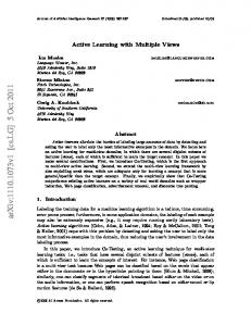
This is known as the ‘cold start problem’ and is a well-known problem in online learning5 . We can see in this figure that the uncertainty sampling and active evidence instance selection perform approximately equally well (i.e. the increase from the baseline is fast, and after querying approximately five instances, the change in classification performance is minimal). We believe the reason for the high classification performance is because selected features are good discriminators between the activities (even though the features selected represent a small subset of the total feature set suggested in [23]). Figure 4 shows the posterior weights that were learnt from the source domain. The mean of the posterior is indicated with the blue bars, and the standard deviation of the weight is shown with the red error bars. We can see from this image that the uncertainty over the weights is quite small in many examples. We also note that higher certainty tends to coincide with smaller absolute posterior mean. By incorporating these posteriors as priors for active learning, we obtain the classification accuracy shown in Figure 3. In this image we can see that without seeing any data the baseline classification performance is approximately 0.75; a significant improvement over the results in Figure 2. Further to the initial improvement in classification accuracy, we can see that the variance over the test subjects is generally lower (most notably with the random selection methods). We also note that the ‘trajectory’ of the classification performance is smoother with active learning. This is likely due to the more principled initialisation of classification weights with transfer learning as new instances will make a smaller overall contribution to the parameters L . In all cases, we see that the evidence-based instance selection achieves better classification performance than random selection in terms of the initial performance increase, steady state classification accuracy, and classification variance over the test subjects. 5

Note that the following images present the shaded regions of the following images represents the standard deviation of the classification, as computed on the full set of target individuals.

Bayesian Active Learning with Evidence-Based Instance Selection

11

Previous work has shown that other selection criteria (e.g. Value of Information (VOI) [25]) are also competitive with uncertainty sampling on this dataset. In order to further investigate the utility of evidence-based instance selection, we calculated the Brier score [26], which is a measure of classifier calibration and found that the the classification models learnt with evidence-based instance selection. Lower mean Brier scores were computed for evidence-based selection than for random sampling and for uncertainty sampling, which is a promising result.

6

Conclusions and Future Work

As we have seen, the activity recognition in the smart-home setting provides challenges in terms of changes in the deployment context and accurate labelling of training data. The natural solution to this is a combination of active learning and transfer learning. We have argued that hierarchical Bayesian methods are particularly well suited to problems of this nature. We then introduced a new active learning method that is based on on Bayesian model selection, and hence fits more concomitantly with the Bayesian framework than previous decision theoretic approaches. We have shown that it outperforms simple random sampling, and is able to cope with situations that the simple but na¨ıve method of uncertainty sampling cannot, in particular when measured by calibration loss. Whilst the proposed method of evidence-based active learning is much more expensive to compute, for our purposes computational burden at the active learning stage is not a pressing issue. Indeed, we find the results of this work promising and believe that low-complexity approximations to our approach may be implemented.

Community weights

50

Feature

40

30

20

10

0

Posterior 2.0

1.5

1.0

0.5

0.0

0.5

weight

1.0

1.5

Fig. 4: Posterior weight distribution.

2.0

2.5

12

Niall Twomey, Tom Diethe, and Peter Flach

We provide some experimental results combining two publicly available activity recognition from accelerometry data-sets, where we transfer from one data-set to another before performing active learning. This is initial work, and our next steps will be to further develop the role of model evidence for instance selection in active learning empirically and theoretically. We will also deploy the various active labelling methods in the prototype smart home, which will allow us to test the active learning framework, as well as the resident-to-resident transfer method. The house-to-house fusion and transfer on multi-modal sensor network can only be tested when multiple homes are available which will be the focus of future work.

Acknowledgement This work was performed under the Sensor Platform for HEalthcare in Residential Environment Interdisciplinary Research Collaboration funded by the UK Engineering and Physical Sciences Research Council, Grant EP/K031910/1.

References 1. C.M. Bishop. Model-based machine learning. Phil Trans R Soc A, 371, 2013. 2. David A. Cohn, Zoubin Ghahramani, and Michael I. Jordan. Active learning with statistical models. J. Artif. Intell. Res. (JAIR), 4:129–145, 1996. 3. Alnur Ali, Rich Caruana, and Ashish Kapoor. Active learning with model selection. In Proceedings of the Twenty-Eighth AAAI Conference on Artificial Intelligence, July 27 -31, 2014, Qu´ebec City, Qu´ebec, Canada., pages 1673–1679, 2014. 4. Sambu Seo, Marko Wallat, Thore Graepel, and Klaus Obermayer. Gaussian process regression: Active data selection and test point rejection. In Mustererkennung 2000, pages 27–34. Springer, 2000. 5. Andreas Krause and Carlos Guestrin. Nonmyopic active learning of Gaussian processes: An exploration-exploitation approach. In Proceedings of the 24th International Conference on Machine Learning, ICML ’07, pages 449–456, New York, NY, USA, 2007. ACM. 6. Neil Houlsby, Ferenc Huszar, Zoubin Ghahramani, and M´at´e Lengyel. Bayesian active learning for classification and preference learning. CoRR, abs/1112.5745, 2011. 7. Shervin Javdani, Yuxin Chen, Amin Karbasi, Andreas Krause, Drew Bagnell, and Siddhartha S. Srinivasa. Near optimal Bayesian active learning for decision making. In Proceedings of the Seventeenth International Conference on Artificial Intelligence and Statistics, AISTATS 2014, Reykjavik, Iceland, April 22-25, 2014, pages 430–438, 2014. 8. Sinno Jialin Pan. Transfer learning. In Data Classification: Algorithms and Applications, pages 537–570. 2014. 9. Parisa Rashidi and Diane J. Cook. Activity knowledge transfer in smart environments. Pervasive Mob. Comput., 7(3):331–343, June 2011. 10. Kyle Dillon Feuz and Diane J. Cook. Heterogeneous transfer learning for activity recognition using heuristic search techniques. Int. J. Pervasive Computing and Communications, 10(4):393–418, 2014. 11. Manfred Opper. On-line learning in neural networks. chapter A Bayesian Approach to On-line Learning, pages 363–378. Cambridge University Press, New York, NY, USA, 1998.

Bayesian Active Learning with Evidence-Based Instance Selection

13

12. Aaron Wilson, Alan Fern, and Prasad Tadepalli. Transfer learning in sequential decision problems: A hierarchical Bayesian approach. In Unsupervised and Transfer Learning Workshop held at ICML 2011, Bellevue, Washington, USA, July 2, 2011, pages 217–227, 2012. 13. Mehmet G¨onen and Adam A. Margolin. Kernelized Bayesian transfer learning. In Proceedings of the Twenty-Eighth AAAI Conference on Artificial Intelligence, July 27 -31, 2014, Qu´ebec City, Qu´ebec, Canada., pages 1831–1839, 2014. 14. Lili Zhao, Sinno Jialin Pan, Evan Wei Xiang, ErHeng Zhong, Zhongqi Lu, and Qiang Yang. Active transfer learning for cross-system recommendation. In Marie desJardins and Michael L. Littman, editors, Proceedings of the Twenty-Seventh AAAI Conference on Artificial Intelligence, July 14-18, 2013, Bellevue, Washington, USA. AAAI Press, 2013. 15. Liu Yang, Steve Hanneke, and Jaime G. Carbonell. A theory of transfer learning with applications to active learning. Machine Learning, 90(2):161–189, 2013. 16. David Kale and Yan Liu. Accelerating active learning with transfer learning. In Data Mining (ICDM), 2013 IEEE 13th International Conference on, pages 1085–1090. IEEE, 2013. 17. T. Diethe, N. Twomey, and P.J. Flach. Bayesian active transfer learning in smart homes. In ICML Active Learning Workshop 2015, 2015. 18. Ralf Herbrich, Thore Graepel, and Colin Campbell. Bayes point machines. Journal of Machine Learning Research, 1:245–279, January 2001. 19. Steven N Goodman. Toward evidence-based medical statistics. 2: The Bayes factor. Annals of internal medicine, 130(12):1005–1013, 1999. 20. Thomas P Minka. Expectation propagation for approximate bayesian inference. In Proceedings of the Seventeenth conference on Uncertainty in artificial intelligence, pages 362–369. Morgan Kaufmann Publishers Inc., 2001. 21. Kevin P Murphy. Machine learning: a probabilistic perspective. MIT press, 2012. 22. T. Minka, J.M. Winn, J.P. Guiver, S. Webster, Y. Zaykov, B. Yangel, A. Spengler, and J. Bronskill. Infer.NET 2.6, 2014. Microsoft Research Cambridge. http://research. microsoft.com/infernet. 23. Davide Anguita, Alessandro Ghio, Luca Oneto, Xavier Parra, and Jorge L Reyes-Ortiz. A public domain dataset for human activity recognition using smartphones. In European Symposium on Artificial Neural Networks, Computational Intelligence and Machine Learning, ESANN, 2013. 24. M. Zhang and A.A. Sawchuk. USC-HAD: A daily activity dataset for ubiquitous activity recognition using wearable sensors. In ACM Int. Conf. on Ubiquitous Computing Workshop on Situation, Activity and Goal Awareness (SAGAware), 2012. 25. Ashish Kapoor, Eric Horvitz, and Sumit Basu. Selective supervision: Guiding supervised learning with decision-theoretic active learning. In IJCAI, volume 7, pages 877–882, 2007. 26. Glenn W Brier. Verification of forecasts expressed in terms of probability. Monthly weather review, 78(1):1–3, 1950.