MILIS: Multiple Instance Learning with Instance Selection

This article has been accepted for publication in a future issue of this journal, but has not been fully edited. Content may change prior to final publication. IEEE TRANSACTIONS ON PATTERN ANALYSIS AND MACHINE INTELLIGENCE

1

MILIS: Multiple Instance Learning with Instance Selection Zhouyu Fu, Antonio Robles-Kelly Senior Member, IEEE, Jun Zhou Member, IEEE

Abstract Multiple-instance learning (MIL) is a paradigm in supervised learning that deals with the classification of collections of instances called bags. Each bag contains a number of instances from which features are extracted. The complexity of MIL is largely dependent on the number of instances in the training data set. Since we are usually confronted with a large instance space even for moderately sized real-world data sets applications, it is important to design efficient instance selection techniques to speed up the training process without compromising the performance. In this paper, we address the issue of instance selection in MIL. We propose MILIS, a novel MIL algorithm based on adaptive instance selection. We do this in an alternating optimisation framework by intertwining the steps of instance selection and classifier learning in an iterative manner which is guaranteed to converge. Initial instance selection is achieved by a simple yet effective kernel density estimator on the negative instances. Experimental results demonstrate the utility and efficiency of the proposed approach as compared to the state-of-the-art. Index Terms Multiple Instance Learning, Support Vector Machine, Feature Selection, Alternating Optimisation

I. I NTRODUCTION Multiple-instance learning (MIL) is a paradigm in supervised learning proposed by Dietterich et. al. [1]. It provides a framework for the classification of collections of instances called bags Z. Fu is with the Gippsland School of Information Technology, Monash University, Victoria 3842, Australia. The work presented here was done when Z. Fu was with the National ICT Australia (NICTA). A. Robles-Kelly, and J. Zhou are with NICTA, Canberra Research Laboratory, ACT 2601, Australia. NICTA is funded by the Australian Government as represented by the Department of Broadband, Communications and the Digital Economy and the Australian Research Council through the ICT Centre of Excellence program. July 2, 2010

Digital Object Indentifier 10.1109/TPAMI.2010.155

DRAFT

0162-8828/10/$26.00 © 2010 IEEE


2

instead of individual instances. In a typical binary MIL problem, the training data are presented in the form of bags and their associated binary labels. The key assumption in MIL is that a negative bag only consists of negative instances, whereas a positive bag comprises both positive and negative instances, although the size of the bags can vary. Mathematically, this can be interpreted as taking the maximum over the labels of all instances in the bag given 1 as the label for the positive class and -1 as the label for the negative class. The hidden nature of the instance labels poses great challenges for MIL. In many cases, negative instances may even dominate in a positive bag. As a result, applying conventional supervised classification methods directly to MIL problems often leads to a downgraded performance [2]. Hence, special-purpose methods have to be designed to handle the MIL problems making use of the structure of MIL. Many problems in computer vision and machine learning can be naturally cast in an MIL setting. For instance, in contents-based image retrieval (CBIR) [3], each image contains many regions, but only those that carry category specific information are of interest (ROI) for purposes of recognition. A ROI can either be a target object in the scene or a region describing the context of the object, provided that it is relevant in the determination of the desired image class. Other regions may be shared across different categories and, therefore, possess no discriminative power. From this viewpoint, an image is a bag and the image regions are instances of the CBIR problem. MIL techniques can also be used for image-level image labelling where a feature vector can be extracted at each pixel and a label is assigned to the whole image aggregating the information gathered from pixel level. One potential problem that hinders the efficiency of MIL is the possible large number of instances encountered in real-world applications. For ROI based image retrieval and object recognition, the training data set may consist of a large number of images, and each image may also contain many ROIs corresponding to the instances, thus the total number of instances involved during the training stage could be prohibitively large. By the assumption of MIL, many instances in the positive class are background instances from the negative class and hence do not contribute much to discrimination. How to efficiently and effectively prune the large set of instances and keep the useful ones still remains an challenging problem for MIL. In this paper, we propose an MIL method with Instance Selection (MILIS). The proposed algorithm is efficient in training and well suited for large scale MIL problems. The method presented here has three major advantages. Firstly, it employs an efficient and robust method for July 2, 2010

DRAFT


3

instance selection based on the distribution of negative instances. Secondly, it uses a single instance representation for each bag similar to MILES [4] albeit with much reduced dimensionality. This is mainly due to the use of a chosen subset of instances for bag-level feature computation in contrast to the use of all training instances as in MILES [4]. The classifier is then optimised by intertwining instance selection with classifier learning in an alternating optimisation framework which is guaranteed to converge. Thirdly, due to the reduced complexity of the algorithm, for the data sets under study, the resulting classifier achieves comparable classification accuracies while being more efficient than alternative SVM-based classifiers for MIL. The rest of the paper is organised as follows. In Section II, we review the relevant MIL literature. We outline the important issues related to the topic and examine the limitations of the existing approaches. In Section III, we formally define the notation for the proposed MILIS algorithm. The details of the algorithm are then elaborated upon in Section IV by introducing the key components of MILIS and showing their integration into an iterative framework. Extension of the algorithm to multiclass settings and a computational complexity analysis are described in Section V. To illustrate the efficiency and effectiveness of the the proposed approach, in Section VI, we report the experimental results on four synthetic and real-world data sets. Finally, we draw conclusions in the last section of the paper and discuss future work on this topic. II. R ELATED W ORK Many methods have been proposed to solve MIL problems. These methods can be roughly divided into two main categories - generative and discriminative approach. Generative approaches dominate in early attempts to tackling MIL problems, which aim at locating a region of interest in the instance feature space such that all positive instances lie in its vicinity and all negative instances are far removed from it. This can usually be cast in a maximum likelihood setting. Dietterich et.al. [1] used axis parallel hyper-rectangles to represent such regions with high positive probability. Maron et.al. [5] proposed Diverse Density (DD), an elliptic target concept in feature space closely related to the peak density of positive instances. In [6], Zhang et.al. proposed EMDD, an alternative to DD using the EM algorithm to locate the target concept in a more efficient manner. This was further generalised to GEM-DD by Rahmani et.al. [7] that keeps multiple hypothesis of the target concepts and hence can achieve improved robustness in locating them. MIL problems can also be tackled in a discriminative manner aiming at adapting standard July 2, 2010

DRAFT


4

supervised learning approaches. For instance, Citation K-nearest neighbour (KNN)[8] extends the standard KNN classifier to MIL by employing the K-neighbours at both, the bag and instance levels. Other variants hinge in the use of Support Vector Machine (SVM) classifiers [9], which result in a plethora of SVM based methods for MIL, which include MI-kernel [10], MI-SVM [11], mi-SVM [11], DD-SVM [3], MILES [4] and other instance level SVM formulations [12], [13], [14]. Other classifiers, which generalise the single instance counterparts above can also be adopted. These include MI-Boosting [15], MI-Winnow [16] and MI logistic regression [2], [17]. Alternatively, we can divide the existing approaches to MIL into top-down and bottom-up ones. Top-down approaches try to infer the bag label directly. During the inference process, additional cues can be gathered to infer the instance labels in a further inference step [4]. Bottom-up approaches work by first inferring the instance labels and then resolving those corresponding to the bags. Generative approaches to MIL are normally bottom up in nature, since the inference process is often effected in the instance feature space. Discriminative approaches, on the other hand, are mostly top down ones addressing bag-level predictions directly. An alternative to this approach is the mi-SVM [11] and akin methods [12], [13] that perform instance inference directly through a generalisation of the maximum margin rationale used in SVMs. The main argument leveled against the bottom-up generative approaches is the use of single or limited number of prototypes to represent the target concepts for the positive class. Despite their empirical success, DD-based approaches rely on a strong assumption that all positive instances form a compact cluster in the feature space. This cluster is exclusive with respect to the collection of negative instances. This is, however, not necessarily the case in real applications as the distributions of positive instances can be arbitrary, and most likely, multi-modal. Hence, a single target concept in the feature space may be insufficient for capturing the distribution of the positive class. Methods such as DD-SVM [3] and GEM-DD [7] remedy this problem by employing multiple prototypes obtained with different start values through iterative optimisation approaches. This motivates our observation that multiple prototypes can be formed and updated iteratively. This delivers robustness to perturbations in the instance feature space due to the aggregation of instance level reasoning.

July 2, 2010

DRAFT


5

Training Data + − − {B1+ , . . . , Bm + , B1 , . . . , Bm− }

Instance Pruning (t=0)

?

Instance Prototypes ∗(t) xi ∈ Bi+ , i = 1, . . . , m+

?

Bag Features ∗(t) ∗(t) zi = (s(Bi , x1 ), . . . , s(Bi , xm+ )) Classifier Training ?

SVM Model f (z) =

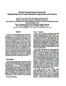
Fig. 1.

i

wi K(zi , z) + b

Instance Updating (t=t+1)

Feature Mapping

Testing Data B Feature Mapping ?

Bag Feature ∗(t) zi = (s(B, x1 ), . . . , s(B, x∗(t) m )) Classification ?

i

Classifier Output wi K(zi , z) + b → f (z)

Block diagram for the proposed algorithm. Left-hand Column: Training Phase; Right-hand Column: Testing Phase

III. P RELIMINARIES AND A LGORITHM OVERVIEW To describe MILIS, we need to introduce some notation. Denote X tr = {X1 , . . . , Xn } as the set of bags and Y tr = {y1 , . . . , yn } as the labels associated with each bag. A bag Xi contains mi instances denoted by xi,j for j = 1, . . . , mi . Without ambiguity, xi,j also denotes the feature vector for the instance depending on the context. Different bags can have different numbers of instances, hence mi may vary for different bags. Each instance xi,j is also associated with a label yi,j which is not directly observable. The assumption is that all instances in negative bags are negative and at least one instance is positive in each positive bag. The purpose is, therefore, to predict the label value for the novel test bag X = {x1 , . . . , xl }. With the above ingredients, we can now describe the MILIS framework for MIL. We first focus on the binary classification case where the label value yi ∈ {−1, 1} for each bag i, where yi = 1 if the bag indexed i corresponds to the positive class and yi = −1 otherwise. By just a few minor modifications, we will later generalise the framework to handle multiclass MIL problems. The basic steps of the MILIS algorithm is illustrated in Figure 1, where each block represents an object to operate on. Each arrow indicates an operation defined on the objects. In

July 2, 2010

DRAFT


6

the training phase, we first perform instance selection on the training instances. This is achieved by modelling the distributions of negative instances and picking the least negative one from each positive bag. After doing this, we obtain a set of Instance Prototypes (IPs), which we denote ∗(t)

by xi . Each of these is chosen from the corresponding positive bag. We then convert the MIL problem into a single instance problem via a similarity based feature mapping using the selected IPs. A single feature vector is formed per bag. In the figure, zi denotes the computed ∗(t)

feature vector for the ith bag, and s(Bi , xj ) denotes the jth feature element which captures ∗(t)

∗(t)

the similarity between bag Bi and instance xj . The explicit form of s(Bi , xj ) will be given in the context that follows. This feature map is in accordance with the single instance feature representation proposed by MILES [4]. Given the bag-level feature vectors, a standard linear SVM classifier is trained on the bag features. Based on the classification results on the training data, we update and reselect the IPs. This step-sequence is interleaved until convergence. In the testing phase, we commence by extracting the feature vector for the test bag using the feature mapping defined over the IPs obtained in the training phase. The trained SVM classifier is then applied so as to obtain the classification result. It is worth noting that instance selection has been addressed previously in a different context. SVM based approaches to MIL such as MI-SVM and mi-SVM [11] perform instance selection to train a SVM classifier in the instance feature space. In contrast, the proposed MILIS algorithm employs instance selection to form the single instance feature representation at the bag level. In this way, the original MIL problem is converted into a prototype selection one. Thus, the purpose of instance selection in MILIS is to construct a more discriminative feature map for learning bag-level classifiers, whereas MI-SVM and mi-SVM aim at selecting the true positive instances for learning instance-level classifiers. IV. I NSTANCE S ELECTION AND C LASSIFIER L EARNING In this section, we present the foundations of MILIS. Like MILES [4], our method aims at solving bag labels directly without resorting to instance level learning in the training process. Note that MILES [4], directly constructs bag-level features based on bag-to-instance distances. Each instance is used to form the bag-level feature mapping and treated as a potential target concept carrying category information, which we term as IP in the context that follows. This gives rise to a very high-dimensional feature vector, whose dimensionality is given by the total July 2, 2010

DRAFT


7

number of instances. Feature selection on these vectors is done implicitly via a one-norm linear SVM, which is known to produce sparse solutions for feature weights [18]. Although effective, MILES has difficulty scaling up to large data sets due to the fact that the dimensionality of the instance feature space is given by the sum of all instances across all bags and, hence, grows linearly with respect to the number of training instances. This leads to high complexity for both feature computation and one-norm SVM optimisation. To achieve comparable performance to MILES with much less computational complexity, explicit instance pruning and selection is necessary. Hence, a principled way is required to reduce complexity devoid of clustering or quantisation procedures. This is an important observation since clustering and quantisation do not consider bag-level structure nor discriminative information and may discard small clusters in the feature space where informative features may be located. Hence we adopt a similar feature representation as MILES which will be described below and at the same time the importance of instance pruning for efficient MIL is highlighted. We then propose a novel discriminant pruning scheme based on density estimation. Next the problems of feature learning and instance updating are addressed. Finally, we summarise the algorithm and provide some theoretical study on its property and computational complexity. A. Bag-Level Feature Representation To effectively employ the similarity based feature mapping in Figure 1, a distance metric needs to be defined first between bags and instances. The Hausdorff distance is a natural distance metric for this purpose. Specifically, the distance between bag Bi and instance x is given by d(Bi , x) = min ||xi,j − x||2 xi,j ∈Bi

(1)

which is the distance between x and its nearest neighbour in Bi . Given the distance metric above, we can then derive the following similarity measure using an exponential function, s(Bi , x) = exp (−λd(Bi , x)) = max exp (−γ||xi,j − x||2 ) xi,j ∈Bi

(2)

If instance x is a true positive instance, then a positive bag should have high similarity to instance x. A negative bag, on the other hand, has a low similarity, since all instances in the negative bag are far apart from x. July 2, 2010

DRAFT


8

Recall that MILES uses all instances in the training set directly to construct the bag-level feature vector. The resulting feature vector for bag i is an m-dimensional vector comprised by the concatenated bag-to-instance similarities ziMILES = [s(Bi , x1,1 ), . . . , s(Bi , x1,m1 ), . . . , s(Bi , xn,1 ), . . . , s(Bi , xn,mn )] where m =

n

i=1

(3)

mi is the total number of instances in the training data set. The subset of input

instances is then selected indirectly by solving a one-norm sparse linear SVM and eliminating the feature dimensions corresponding to zero classifier weights. Despite its flexibility and robustness, the above feature mapping scheme often leads to a computationally expensive training process. The reasons are two-fold. First, the feature mapping results in full-length features whose dimensionality is given by the total number of instances in the training set. Even for moderately large data sets, this could still be a large number. Furthermore, the feature matrix is not sparse. In order to calculate a single entry of the feature matrix, a nearest neighbour search between features of the prototype instance and those in the bag under study is required. This consumes not only many computational resources but a lot of storage. Second, there is no efficient method to solve the one-norm SVM except from solving its linear programming (LP) formulation. This becomes the bottleneck in the efficiency of the MILES. For some large-scale MIL data sets, even commercial LP solvers can be very slow or even inapplicable. Thus, it would be desirable to design an alternative approach that can reduce the computations in both feature mapping and classifier learning, while at the same time, exploiting the single instance feature representation of MILES. B. Initial Instance Selection As discussed earlier, DD-based instance selection is computationally expensive, as it involves solving an unconstrained optimisation problem for every instance in the training set in order to recover all the prototypes corresponding to the DD extrema. Instead of using all training instances to form the bag-level feature vector in Equation 3, DD-SVM chooses a set of prototypes to construct the feature map. The prototypes are obtained by running EM-DD [6] from different initial points. In this section, we propose an efficient approach to instance selection for the construction of bag-level feature map. We select existing instances in the training set to construct the similarity July 2, 2010

DRAFT


9

based feature. This is equivalent to taking columns of the MILES feature representation in Equation 3. To construct bag-level feature vectors, a single instance is selected from each training bag to form the subset of instance prototypes (IP) for feature mapping. Intuitively, we want to include true positive and negative instances in the subset to compute a discriminative feature map. Note that, following the MIL assumption, everything in the negative bag is negative. Hence the key problem here is to locate the true positive instances. While DD-based selection approaches tries to consider true positive instances directly and attempting to locate regions in the feature space with high positive density, it is much more effective to model the distribution of the negative population. Since negative instances can have very general distributions, to model all instances contained in the negative bags we use the following Gaussian kernel based Kernel Density Estimator (KDE) [19] f (x) = where

x− i,j

Z

1 i

mi

mi

exp −β||x − x− i,j ||

(4)

yi =−1 j=1

denotes the jth instance from the ith negative bag, Z is a normalisation factor making

f (x) a proper density. It is constant over the instance space and is thus ignored in our calculation. We have employed an isotropic Gaussian kernel with the scale parameter β controlling the range of influence for training instances. Notice the above equation defines a normalised probability density function (PDF) for the negative population. The major advantage in modelling the negative population in this manner resides in the fact that, due to their large quantities, negative instances usually dominate the joint PDF in MIL settings. Their distributions can then be modeled more accurately than true positives making use of KDE. To achieve an efficient density estimation for each positive instance, we pick its K-nearest negative instances and evaluate the probability of the positive instance being generated from the negative population via Equation 4. The search process can be accelerated by using the approximate KNN search method in [20]. We then pick the single instance with the lowest likelihood value, i.e. the least negative instance, from each positive bag as the IP. For each negative bag, on the other hand, we pick the single instance with the highest likelihood value, i.e. the most negative instance, as the IP used in the feature mapping. The total number of IPs obtained is equal to the number of bags. This compares quite favorably with the number of prototypes used in MILES, which is equivalent to the set of all training instances. This results July 2, 2010

DRAFT


10

in a much lower-dimensional feature space without much loss of discriminatory power, as each bag is represented by a corresponding instance selected from the bag. Compared to DD based selection, we also obtain improved IPs in a more computationally efficient manner. Furthermore, since our instance selection method is governed by PDFs, it is more robust to noise corruption and outliers in the data set. Finally, as we will see later, the above instance selection procedure can be generalised to the multiclass MIL case. The complexity is solely determined by the number of instances and is independent of the number of classes. C. Classification After initial instance selection, we have obtained a subset of instance prototypes {x1 , . . . , xn }, where xi is the prototype selected from the ith bag in the training set. The bag-level feature is then given by zi = [s(Bi , x1 ), . . . , s(Bi , x2 ), . . . , s(Bi , xn )]

(5)

where s(Bi , xj ) is computed via Equation 2. We then train a classifier that can be applied to the bag features. To this end, we use linear SVM which employs the L2 norm for both the regularization term on feature weights w and the data term as follows 1 f (w) = ||w||2 + C (yi , wT zi ) 2 i

(6)

(yi , wT zi ) = (1 − yi wT zi )2+ where yi ∈ {−1, 1} is the label value for bag i, C is the regularisation parameter that controls the influence of the second term on the right-hand side of the above equation. The resulting classifier is given by wT z, where w are the linear weights for the features. Here, we have also absorbed the bias term into the weight vector w for the sake of simplicity. (yi , wT zi ) specifies the loss function for classification, where (v)+ = max (0, v) is the Hinge loss normally adopted for SVM classifiers. The reason for the use of L2 linear SVM here responds to computational efficiency. Unlike one norm SVMs, which are solved by standard linear programming optimisation routines and do not scale up with training sample sizes, two norm SVMs have been well studied in the literature. There are fast routines to solve the underlying quadratic program for two-norm SVMs [21], [22] July 2, 2010

DRAFT


11

using linear and nonlinear kernels. Linear SVMs can be trained in an efficient manner using various methods proposed in the literature [23], [24]. Note that we can also use a nonlinear SVM classifier here. Nonetheless, there are several advantages for using linear SVMs aside from efficiency alone. Firstly, linear SVMs can be used for implicit feature selection. We can discard feature dimensions with small coefficients in the classifier weight w, thus, effectively further reducing the number of instances used in constructing the feature mapping. SVMs with nonlinear kernels such as the RBF one, do not have this property for feature selection. All feature dimensions are treated equally in the computation of nonlinear kernels. Secondly, the feature mapping defined in Equation 5 is itself nonlinear in nature due to the use of exponential operator that maps distances to similarities. It defines a higher dimensional embedding in the original feature space via this nonlinear mapping. Consequently, a linear classifier suffices to separate features which are not linearly separable in the original feature space. D. Instance Update After obtaining the SVM classifier for bag-level features, we can validate the selected IPs and update them accordingly. This can be cast as an optimisation problem over discrete variables that can be efficiently solved using an approach akin to coordinate descent. To introduce the optimisation problem, we define a set of auxiliary variables φi , where i = 1, . . . , n for each bag in the training set. Each φi can take values in {1, . . . , mi } and φi = j implies the jth instance in the ith positive bag is selected as the IP for the feature mapping. With these ingredients, we now define the optimisation problem underlying the iterative framework in terms of the variables φi and the classifier weights w as follows 1 (yi , wT g(Bi , φ)) min Q(w, φ) = ||w||2 + C w,φ 2 i

(7)

g(Bi , φ) = [s(Bi , x1,φ1 ), . . . , s(Bi , xn,φn )] where (yi , fi ) is the same loss function as defined in Equation 6, and g(Bi , φ) specifies the baglevel feature mapping for the ith bag Bi given the indices of the prototypes φ = {φ1 , . . . , φn }. Given the trained SVM classifier with weights w, we can further update the IP for each bag. This is equivalent to minimising Q(w, φ) in Equation 7 with respect to φ. We adopt a reminiscent procedure of coordinate descent so as to update φi for each bag as follows July 2, 2010

DRAFT


12

(t+1)

φ1

m1

= arg min j=1

(wT g(Bi , {j, . . . , φ(t) n }), y1 )

(8)

i

... (t+1)

φi

mi

= arg min j=1

(t)

(t)

(wT g(Bi , {. . . , φi−1 , j, φi+1 , . . .}), yi )

i

... mn

φn(t+1) = arg min j=1

(t)

(t+1)

where φi and φi

(t)

(wT g(Bi , {φ1 , . . . , j}), yn )

i

correspond to the old and updated index values for the ith bag respectively,

w is fixed to w(t) for the tth iteration. Since w is unchanged during the update of φ, only the second term on the right-hand side of Equation 7, i.e. the data term of the SVM objective function, is considered here. Each φi is updated while fixing all other φ’s. We can see that each update of the IPs leads to a lower cost for the SVM data term and, hence, decreased upper bound on the classification error. The order for which the IPs are updated is not fixed and can be shuffled randomly. Here, we choose an ordering scheme such that IPs for misclassified bags are updated first. In our experiments, this scheme has delivered good performance. Despite the simple procedure of the instance update algorithm, a naive implementation may lead to a very time consuming computational process. This involves calculating the bag-toinstance affinity between each bag in the training set and every training instance except those currently chosen as the IPs. This has the same time complexity as computing the full MILES feature embedding. Thus, following each such update, the bag-level feature values are changed. This implies that the decision values need to be re-evaluated for each training example. Fortunately, we can avoid the above computationally expensive steps by taking advantage of the incremental nature of the instance update process. We make use of two important observations here. Firstly, the update of each φi would result in the change of the ith feature element for the bag-level feature mapping while all other feature dimensions are unaffected. Hence, instead of re-calculating the classifier output for the new feature vector, we can update the classifier output incrementally based on the change in the ith feature alone. Secondly, empirical observations show that only a few training instances are discriminant for the MIL problems we are studying. This is especially true for the case of positive bags with many instances, in which the majority of the instances are false positives bearing little discriminant information. Hence, many training July 2, 2010

DRAFT


13

instances, if chosen as prototypes, will contribute to a higher cost function value. Therefore we can update the feature map and the classifier output simultaneously and stop the update process early on if the new feature map yields solution that depart from the current optimum. The pseudo-code of the instance update algorithm can be found in Figure 2, where B, Y , Z (t) , φ(t) and w are the training data, training labels, current feature map, indices of prototypes currently selected, and the classifier weights, respectively. The algorithm outputs the updated feature map Z (t+1) and the new indices of prototypes φ(t+1) . The basic flow of the algorithm should be self-explanatory from the pseudo-code. The ”feature update” subroutine adopts the above mentioned strategies within the for loop, where new classifier output i is updated from the current output fi , and each iteration is stopped early if the cost function value v for the new feature map (evaluated up to the current bag) is suboptimal with respect to the current value of v. E. Iterative Learning Framework The two steps of classifier training and instance selection can be interleaved in an twostep optimisation fashion. Once a classifier is trained, we can update the IPs. Then a new classifier can be learned from the updated feature mapping. This can be viewed as minimising the optimisation problem defined in Equation 7 over continuous and discrete variables. The initial instance selection process discussed in Section IV-B corresponds to the initialisation of φ. While SVM training corresponds to optimisation with respect to w while fixing φ, the instance update process discussed in the previous section is equivalent to minimising φ while fixing w. It is straightforward to see that each iteration decreases the value of the cost function in Equation 7 according to the following relation f (w(t) , φ(t) ) ≤ f (w(t+1) , φ(t) ) ≤ f (w(t+1) , φ(t+1) )

(9)

where w(t) and φ(t) refer to the old classifier weights and the indices of prototypes in each bag, while w(t+1) and φ(t+1) correspond to new classifier weights and indices of IPs. The first inequality holds due to the classifier updating step and the second inequality arises from instance updating. Because of the monotonic decrease in energy, the iterative learning framework is guaranteed to converge in a finite number of steps. Moreover, since φ can only take a finite set of values due to the discrete nature of the φi variables, this updating process is guaranteed to July 2, 2010

DRAFT


14

Fig. 2.

Pseudo-code for Instance Update

July 2, 2010

DRAFT


15

(t+1)

converge towards φi

(t)

= φi for every i. That is, at convergence, the IPs selected from two

adjacent iterations do not change. The above procedure is reminiscent of the EM algorithm [25], which aims at recovering maximum likelihood solutions to problems involving missing or hidden data by iterating between two computational steps. In the E (expectation) step we estimate the a posteriori probabilities of the hidden data using maximum likelihood parameters recovered in the preceding M (maximisation) step. The M-step in-turn aims to recover the parameters which maximise the expected value of the log-likelihood function. Despite their similarity, the underlying nature of the method proposed here and the EM algorithm are quite different. Firstly, from the statistical point of view, the EM algorithm provides a means for maximum likelihood parameter estimation in the presence of hidden variables. In contrast, the target function in Equation 7 for our method is tailored to the setting of the MIL problem being considered and is not related to the likelihood function or a particular expression of the a posteriori probabilities. Secondly, from the optimisation point of view, the EM algorithm is well-known as a bound optimisation technique that maximises a concave lower bound on the likelihood function at each iteration [26]. Our method, on the contrary, is a minimiser of the target function without resorting to a lower bound.

Fig. 3.

Summary of the proposed iterative framework for instance selection and classifier learning

The step-sequence of the iterative framework for instance selection and classifier learning

July 2, 2010

DRAFT


16

is outlined in Figure 3. In the algorithm above, after the SVM classifier is trained in the last iteration, we adopt a final feature pruning step by removing all features with small feature weights. Since these features have a small contributions to the final output of the linear classifier, the classification performance does not suffer from removing these redundant instance features. Specifically, the jth feature is removed if the magnitude of its corresponding feature weight is small, that is |wj | < r for some small r > 0. The threshold r can best be determined relative to the scale of the feature weights by some simple statistics, such as the mean and the median of the feature weights. As we will see in the experimental section, the performance of the proposed method is not sensitive to the choice of the value of r. Note that the strategy used here is similar to the recursive feature selection technique for SVM [27], which also uses feature weights obtained from the SVM classifier as indicators for their discriminabilities. Instead of removing a single instance feature and retraining the SVM at each iteration, we make use of the threshold r and prune multiple features in the space at every step of the algorithm. This final step results in further instance pruning by removing the indiscriminate instance prototypes as indicated by the classifier weights. Since each feature in the feature map corresponds to one selected prototype, after removing those redundant prototypes, the feature map can be updated and the SVM classifier re-trained based on the updated instance feature matrix. In this way, we can improve on the efficiency of testing without influencing the performance, since prediction time is monotonic to the number of instances used to form the feature mapping. The algorithm in Figure 3 can also be formulated in a one-norm SVM framework simply by replacing the standard SVM classifier with the one-norm SVM classifier [18], in a similar fashion as MILES [4] and the one norm extension of MI-SVM [14]. The training of SVM classifier becomes a standard linear program and the instance update procedures can also be modified accordingly. With the one-norm formulation, feature selection can be achieved in an implicit manner since the L1 norm imposes sparsity on the learned feature weights. However, two major disadvantages hinder our further consideration of this alternative. Firstly, it may still be computationally expensive to solve the linear program arising from the one-norm formulation, whose complexity scales with the number of bags in the training set. It may be costly to solve the new one-norm SVM formulation if the MIL problem contains a large number of bags. However, this is not a problem for SVMs with squared norms, where there exist efficient methods for July 2, 2010

DRAFT


17

training on large data sets [21], [22]. Secondly and more importantly, one-norm SVM, despite its ability for implicit variable selection, does not have any advantage in performance over the standard SVM when incorporated into our MILIS framework. It is worth noting that in our empirical evaluation of MILIS using both standard and one-norm SVMs on the benchmark MUSK and COREL data sets, as mentioned in the experimental section, one-norm SVM delivers inferior classification performances as compared to those produced by squared-norm SVMs. Hence, we still focus our attention on the standard SVM formulation and resort to an additional step of final feature pruning to maintain the sparsity of obtained IPs as discussed above. In the testing stage, given a test bag B, we first form its bag-level feature vector z via Equation 5 using the learned IPs. Prediction is made by taking the sign of the decision value output the linear SVM z = [s(B, x1 ), . . . , s(B, x2 ), . . . , s(B, xn )] f (B) = sgn (wT z)

(10)

V. E XTENSION TO THE M ULTICLASS S ETTING In this section, we show how the algorithm proposed in the previous sections for binary MIL can be generalised to handle multiclass MIL tasks. Unlike traditional approaches that make use of various classifier fusion frameworks to decompose the multiclass problem into several binary ones and combine the results from the binary classifiers for multiclass classification [28], [29], we propose to solve the multiclass MIL problem using a direct formulation of the SVM for multiclass classification problems [30]. For the binary MIL algorithm based on instance selection discussed above, this can be effectively achieved by making some minor modifications as described below. A. Instance Selection For multiclass MIL problems, each class is a positive one against the remaining classes. Hence for each bag in any class, there exists at least one true positive instance carrying the discriminant information for the class under consideration, where the remaining instances may be viewed as “background” ones. For some applications, there might be a number of bags which contain background instances alone, akin to the negative class in the binary case. Note that this change July 2, 2010

DRAFT


18

in the problem formulation does not influence our instance selection framework. The reason for this will soon be apparent. We still use density estimation to evaluate the conditional probability for the distributions of instances for each class. Yet, instead of treating them as the true positive distributions for themselves, we use the class conditional distribution of each class to model the negative distributions for other classes. Denote P (x|Ωk ) the class conditional distribution of training instances from the kth class. An estimate of P (x|Ωk ) can be obtained from kernel density estimation via Equation 4 over all instances extracted from the kth class. Again, in estimating the conditional probabilities of novel instances for the jth class, we first perform a K-NN search to find an appropriate neighbourhood in the jth class before applying Equation 4 for density evaluation. With the class conditional probability values at hand, we then use the following likelihood ratio value defined for the jth instance in the ith bag, xi,j , as an indicator for its discriminability r(xi,j ) =

P (xi,j |Ωyi ) maxk=yi P (xi,j |Ωk )

(11)

where yi ∈ {1, . . . , c} is the label for bag i. The instance with the largest likelihood ratio value in the above equation is selected as the (0)

initial prototype for bag i. That is, φi

= arg maxj r(xi,j ). This is similar to the binary case.

The main difference is in the modelling of the negative distribution for each class. We take the maximum over all other classes for two reasons. Firstly, this is more efficient than running the density estimator over all instances from all other classes. As a result, we end up running KDE for each class only once. Secondly, the maximum of the class conditional probability is a robust indicator for the discriminability. If and only if all other classes have a low density and the current class has a high density over the support region of the instance, can the instance become a prototype that carries the discriminative information for the class it represents. Thus, our multiclass selection strategy provides a seamless way to handle different classes. More importantly, the feature map inferred from the selected IPs is common for all different classes, which makes the following classifier learning and optimisation process more convenient.

July 2, 2010

DRAFT


19

B. Classification Crammer and Singer [30] have proposed a multiclass SVM by solving the following single optimisation problem min f (w1 , . . . , wc ) =

c 1 j=1

2

||wj ||2 + C

(yi , fi )

(12)

i

(yi , fi ) = (1 − (fi,yi − max fi,j ))2+ j=yi

Here c linear classifiers are learned in parallel and fi = [fi,1 , . . . , fi,c ] are the decision values returned by the c linear classifiers. The weight for the kth linear classifier is given by wk and fi,k = wkT xi is the decision value returned by the kth classifier. A testing example is assigned label k if the decision value returned by the kth classifier is larger than those returned by other classifiers. In the above equation, (yi , fi ) represents the generalised squared Hinge loss for multiclass output, which varnishes if and only if fi,yi − maxj=yi fi,j ≥ 1. The use of L+ (.) encourages large margins over wrong decisions for the training data. The second term on the right-hand-side specifies an upper bound on the classification error, whereas the first term is the regularisation term that penalises complicated decision boundaries. C. Instance Update The step sequence of the instance update algorithm remains the same as that presented in Figure 2 except for two minor changes. Firstly, the binary hinge loss term L(fi , yi ) is represented by its multiclass counterpart L(fi,1 , . . . , fi,c , yi ) as defined in Equation 12. Secondly, the two equations for evaluating and updating classifier output values fi in the ”feature update” routine are replaced by the following two equations (t)

fi,k = wkT Zi

fi,k = Fi,k + wj,k (zi,j − zi,j ) for all k = 1, . . . , c. and an additional loop is added to evaluate fi,k and update fi,k

For the final instance pruning after the iterative update of instance prototypes and classifiers, pruning is effected if and only if the corresponding instance feature weights for all c classifiers

July 2, 2010

DRAFT


20

are small. Note that the testing stage shares the same first step as in the binary case. The baglevel feature vector z is formed via Equation 5 using the learned IPs. The bag is then assigned the label corresponding to the largest decision value output by the linear SVM c

f (B) = arg max wjT z

(13)

j=1

where z = [s(B, x1 ), . . . , s(B, x2 ), . . . , s(B, xn )]. VI. E XPERIMENTAL R ESULTS We performed experiments on both synthetic data and real-world data sets to demonstrate the utility of the proposed algorithm. We use synthetic data to show the effectiveness of the MILIS algorithm in instance selection and compare it against EM-DD based selection criteria [6], [3]. We then demonstrate the performance of MILIS for MIL classification on four realworld data sets. To show the generality of the method, we use two binary classification tasks namely drug activity detection and infested plant pathogen detection in hyperspectral imagery. We also used two multiclass classification settings, region based image classification and object class categorisation. For all our experiments, we have fixed the number of iterations of MILIS to 5. The number of iterations was set empirically as a trade-off between the convergence of optimisation and performance improvement. The feature mapping parameter γ in Equation 2 as well as the SVM regularisation parameter C was chosen via 5-fold cross validation on the training data using grid search. The scale parameter β for KDE in Equation 4 was fixed to be equal to γ for both binary and multiclass MIL problems. For drug activity detection and region based image retrieval, we compare the training time of MILIS with the alternative MILES algorithm. The code has been implemented in Matlab with the key routines of instance selection/updating and classifier training written in C++. For the KNN search involved in density estimation, we have used ANN, a C++ library for approximate nearest neighbour searching

1

and empirically set the

number of neighbours k to 10. In practice, we find the results of instance selection are not very sensitive to the choice of k provided k is on the order of 10. The experiments were conducted on a PC with a 3.0GHz Intel Core 2 Duo CPU and 4GB of memory. All algorithms (including MILIS, MI-SVM, mi-SVM, and MILES) were implemented 1

The package can be downloaded at the address http://www.cs.umd.edu/~mount/ANN/

July 2, 2010

DRAFT


21

in house making use of the LIBSVM C++ package for training the 2-norm SVMs [24] 2 . LIBSVM solves the standard SVM using sequential minimal optimisation [21]. We apply LIBSVM only in the first iteration of SVM training to provide an initial value for SVM weights. Subsequent steps use stochastic gradient descent [31] to update the SVM weights in an incremental fashion. For the MILES and MILISL1 implementations, we have used the MOSEK optimisation package 3 so as to solve the LP arising from the one-norm SVMs. Note that, nonetheless the results in [4] where obtained used the CPLEX software for solving the LP, the computation times will ultimately be dependent on the size of the MIL problem at hand. Since complexity grows as a function of the training instance data set, it may not be possible to consistently rely on the power of a fast LP solver to tackle increasingly complex problems arising in the MILES setting [4]. It is worth noting here that we tested other LP packages at our disposal, including the linprog routine in the Matlab optimisation toolbox, the GNU Linear Programming Kit (GLPK) and PCx 4

. We found none of them could outperform the speed of MOSEK in our experiments.

A. Synthetic Data Results We commence by illustrating the ability of instance selection via MILIS for the synthetic data set shown in Figure 4. We have generated a data-set of 20 positive bags and 20 negative ones, with 5 instances in each bag. The instances are represented by circles in Figure 4(a). There is only a single positive instance in each positive bag. The positive instances are randomly drawn from a mixture of Gaussians (MoG) with two components, as shown in broken magenta curves in Figure 4(a). The negative instances are drawn from a different MoG distribution with two Gaussian components shown in broken cyan curves. The solid triangles shows the center locations of the respective Gaussian components. Figure 4(b) shows the IPs extracted by EMDD [6] in red plus signs. We can see that a large amount of IPs lie further away from the data distribution. This is due to the non-convexity of the EM-DD cost function, which is likely to generate outliers with high likelihood value. Figure 4(c) provides a close-up view of the IPs yielded by EM-DD. Figure 4(d) shows the IPs selected by the nonparametric KDE approach in 2

The package can be downloaded at the address http://www.csie.ntu.edu.tw/~cjlin/libsvm/

3

For more information visit http://www.mosek.com/

4

For more information on PCx visit http://pages.cs.wisc.edu/~swright/PCx/

July 2, 2010

DRAFT


22

(a) Raw data

Fig. 4.

(c) EM-DD close-up view Example results of instance selection on synthetic data.

(b) EM-DD

(d) MILIS

MILIS. We can see that MILIS has successfully selected the single positive instance from each positive bag as the initial IP. This is in contrast with the initial IPs selected by EM-DD are not as discriminative as those of MILIS with many miss-hits. Moreover, MILIS takes less than 0.1 seconds for initial instance selection on this data set and is much more efficient than EM-DD, which takes more than 15 seconds and, thus, can be impractical for large-scale applications. We also examined the effect of initialisation on MILIS. In fact, we found it is not overly sensitive to initialisation, which is illustrated on the same data set. We deliberately initialise all IPs to the negative instances. After 5 iterations, the majority of the IPs are updated to the positive instance with classification error dropping to 0. This process is shown in Figure 5, where the top-left panel shows the plots for the initial IPs. Those in the last iteration and the cost function value/error rate as a function of iteration number are shown on the bottom row. Intermediate IPs for iterations 1, 3 and 5 are shown in the remaining panels.

July 2, 2010

DRAFT


23

Fig. 5.

(a) Initial step

(b) Iteration 1

(c) Iteration 3

(d) Iteration 5

(e) Final result (f) Cost (y-axis) vs. iteration number (x-axis) Behavior of IPs as a function of iteration number for poor algorithm initialisation.

B. Drug Activity Detection In our second experiment, we test MILIS on the two musk data sets, MUSK1 and MUSK2 for drug activity prediction. These are the standard benchmark data sets for testing MIL algorithms. Both data sets are accessible from the UCI Machine Learning Repository 5 . The data set MUSK1 contains 92 bags with 47 of them being positive and the remaining 45 being negative. The data set has an average of 5.17 instances in each bag. The data set MUSK2 contains 102 bags where 39 of them are positive and the remaining ones are negative, with each bag having an average of 64.70 instances. Table I reports the classification results measured in terms of the mean prediction 5

http://www.ics.uci.edu/~mlearn/MLRepository.html

July 2, 2010

DRAFT


24

Algorithm

MUSK1

MUSK2

MILIS

88.6: [85.8, 91.5]

91.1: [89.4, 92.8]

MILISL1

85.6: [82.5, 88.7]

88.8: [87.2, 90.4]

MILES [4]

86.3: [84.9, 87.7]

87.6: [86.2, 89.2]

MI-SVM [11]

83.8: [82.6, 84.9]

86.5: [85.0, 88.0]

mi-SVM [11]

88.0: [87.0, 88.0]

88.4: [87.0, 89.8]

DD-SVM [3]

85.8

91.3

APR [1]

92.4

89.2

DD [5]

88.9

82.5

EM-DD [6]

84.8

84.9

TABLE I P ERFORMANCE COMPARISON OF THE MILIS ALGORITHM AND THE ALTERNATIVES ON THE MUSK DATA SETS .

Algorithms

MILIS

MILISL1

MILES

MI-SVM

mi-SVM

MUSK1

0.2 ± 0.1

0.6 ± 0.2

2.6 ± 0.4

0.25 ± 0.05

0.3 ± 0.1

MUSK2

6.8 ± 2.0

12.8 ± 1.0

691.9 ± 292.3

8.3 ± 0.8

13.2 ± 1.8

TABLE II C OMPARISON OF TRAINING SPEED , IN SECONDS , FOR THE MUSK DATA SETS .

accuracy of 10-fold cross validation. Here, we have tested standard MILIS and its variant using one-norm SVM as the classifier, termed MILISL1 in the table. We have also tested MILES, MISVM and mi-SVM and report, in square brackets, the mean cross validation accuracy averaged over 15 different random runs and the 95% confidence interval. For the sake of completeness, we have also included results for other MIL methods in [4]. From Table I, we can observe that MILIS delivers better performance in terms of higher classification accuracies as compared with those yielded by MILES and other alternatives. In Table II, we report the timing results for MILIS and the alternatives. The speedup of MILIS over MILES for the MUSK2 data set is more obvious due to the large number of instances. As mentioned earlier, the main obstacle to the efficiency of MILES is in the training of the one-norm SVM, which could be very costly for large number of instances and leads to the big difference in training speed for the two methods under study. This is also corroborated by the training speed of MILISL1 , where the one-norm SVM classifier takes more time in training than that used for the “standard” MILIS. MI-SVM and mi-SVM are faster than MILES but still

July 2, 2010

DRAFT


25

slower than MILIS when applied to the MUSK2 dataset. This is because they treat the SVM classification problem at the instance level. At each iteration, mi-SVM learns an SVM in the instance feature space using all input instances as the training set. MI-SVM trains a similar SVM by using all negative instances and a single positive instance in each positive bag. Thus, their computational cost increases greatly when the data set contains a large number of instances per bag, which is the case for the MUSK2 data set. Next, we examine the influence of different initialisation strategies on the performance of MILIS. Besides the initialisation using KDE as discussed in Section IV-B, we can also initialise MILIS in three different ways. In the first of these, the initial IPs are selected randomly from the training bags (RANDOM). The second initialisation alternative uses DD values as a guide for the true positivity of the instance (DD). Specifically, let x be an instance in a bag B from the kth class. We can evaluate its DD value making use of the following equation s(Bi , x) (1 − s(Bi , x)) i,yi =k

i,yi =k

and select the instance achieving the highest DD value in the bag as the IP. The final strategy for initialisation is to simply use all instances in the training bag to form the bag-level feature map (ALL), which is the same as the MILES feature map. The only difference here is that a two-norm SVM classifier is used instead of the one-norm SVM. The SVM can be solved more efficiently in its dual formulation with complexity dependent on the number of bags in the training set. Since all instances are used to form the initial feature mapping, there is no need for instance update and iterative learning though. Table III compares the performances achieved by the above-mentioned initialisation strategies for MILIS on the MUSK data sets. From the table, we can see that KDE achieves the highest accuracy on average for the MUSK1 data set and is highly competitive with respect to DD initialisation for the MUSK2 data set. Moreover, the alternative strategies achieve more or less comparable classification accuracies for both data sets. However, non of the alternatives produce a consistently better performance on both data sets in comparison with the proposed KDE instance selection method for initialisation. Finally, we examine the sensitivity of the final feature pruning to the cut-off threshold value r with respect to the classification performance as well as the sparsity of the resulting feature map. Figure 6 shows the classification accuracies in percentage and sparsity values of MILIS against different cut-off values versus those of MILES. Here, the threshold r is a relative cut-off July 2, 2010

DRAFT


26

Initialisation method

MUSK1

MUSK2

KDE

88.58 : [85.71, 91.45]

91.09 : [89.42, 92.76]

RANDOM

86.76 : [82.22, 91.30]

90.19 : [89.01, 91.36]

DD

87.03 : [83.76, 90.30]

89.95 : [88.20, 91.70]

ALL

87.07 : [83.37, 90.76]

91.63 : [90.35, 92.92]

TABLE III P ERFORMANCE COMPARISON OF DIFFERENT INITIALISATION METHODS FOR MILIS ON THE MUSK DATA SETS .

Fig. 6.

(a) MUSK1 (b) MUSK2 Influence of final feature pruning on classification performance and sparsity for MILIS on the MUSK data sets.

value which has been set to multiples of the median of the feature weight absolute values. The sparsity values are computed by the average percentage of final number of IPs corresponding to nonzero weights within the total number of training instances over different training rounds. It can be seen that in contrast to MILES, MILIS not only achieves higher classification accuracies, but also generates sparser feature maps for sufficiently, but reasonably large cut-off values. This leads to higher efficiency in the testing stage. This efficiency of prediction is largely dominated by the time spent on computing the feature map, which is directly relevant to the number of IPs kept after training. We also note that the performance of MILIS is quite insensitive to the choice of cut-off values for a large range of r. Only when r > 2 the performance starts to downgrade noticeably. Hence, in practice its quite easy to empirically select a cut-off value which achieves a good trade-off between performance and efficiency. Here, we have set r = 1 for all our experiments.

July 2, 2010

DRAFT


27

Fig. 7.

(a) (b) (a) Mean Spectra for the instance in all bags (blue), positive bags (red) and negative bags (green); (b) Influence of

final feature pruning on classification performance and sparsity.

C. Plant Pathogen Detection in Hyperspectral Imagery Next, we turn our attention to the detection of plant pathogens via hyperspectral imagery. In this application, we are interested in the use of hyperspectral imagery for crop disease detection and mapping. We have taken 120 images of capsicum plants (CAPS) where 60 of them are healthy. The rest of these have been infected with a virus whose visible symptoms are not yet apparent. The left-hand column of Figure 8 shows sample pseudo-colour images for both healthy and infected specimens. From the colour alone, there is no noticeable difference between the two. Nevertheless, we can classify them based on their hyperspectral signatures. This is a typical MIL problem, where an image is a bag and foreground pixels (i.e. pixels representing plant tissue) are instances in the bag. Healthy plants are referred to as the negative class whereas infected ones are deemed as positive. While healthy plants should have all healthy leaves, not all regions on the infected plant leaves are ill. We use the normalised reflectance at each pixel as the instance level feature vector. Sample foreground regions for the pseudo-colour images are shown in the middle column of Figure 8. In Figure 7(a), we show the mean spectra of all pixels in the ROI for each image, as well as the mean pixel spectra for positive (infected) and negative (healthy) classes. Note that here we have offset the curves for the sake of clarity, otherwise they would all overlap with each other in the figure. From the average statistics, there is no apparent existence of patterns that distinguish the positive class from the negative one. For our experiments, we have randomly divided the image data set into 6 disjoint subsets with equal number of healthy and infected plants. The ROI of each training image contains July 2, 2010

DRAFT


28

(a)

(b) Accuracy

Initialisation method

Performance

Infected Class

93.93 : [92.90, 94.96]

KDE

92.87 : [92.27, 93.47]

Healthy Class

91.24 : [90.09, 92.39]

Random

92.18 : [91.54, 92.82]

Overall

92.87 : [92.27, 93.47]

DD

91.59 : [90.69, 92.50]

All

92.67 : [91.82, 93.52]

TABLE IV ( A ) C LASSIFICATION PERFORMANCE OF MILIS ON CAPS DATA SET; ( B ) P ERFORMANCE COMPARISON OF DIFFERENT INITIALISATION METHODS FOR

MILIS ON THE CAPS DATA SET.

an average of 500 pixels, which is equal to the number of instances in each bag. Hence, the dimension of the instance space is over 20000, making the MILES embedding overly complex for the problem. Yet, MILIS can still be successfully applied. We applied it to the image data set and measured the average 6-fold cross validation accuracy. The above test is repeated over 10 different random partitions. The mean classification accuracy and the standard deviation are reported in Table IV(a). We can see that MILIS is quite effective in detection and achieves an overall accuracy rate of 92.9%. It has a low false positive rate, and in average, over 9.1 out of 10 healthy samples are classified correctly. The detection rate for infested plants is higher, with an average about 9.4 out of 10 infested plants will be identified by our approach. Considering the challenging nature of this application, the results are quite encouraging. Note that this trend is consistent with the previous application. Table IV(b) reports the performance of different initialisation methods, as discussed in the previous section, on the CAPS data set. All four initialisation strategies perform quite similarly for this data set, with KDE achieving a margin of improvement on classification accuracy over the alternatives, followed by initialisation using all instances and random selection of IPs. Instance selection based on DD values does not perform as well as expected. Figure 7(b) shows the plots for classification accuracy and sparsities versus the cut-off threshold. As before, that classification performance is quite stable for a large range of cut-off values. Within this range, sparsity can be maintained by increasing the cut-off value. In the rightmost column of Figure 8, we show the image mapping results rendered by MILIS for both healthy and infected plants. This is achieved by treating each pixel as a bag with singleton instance and applying the learned classifiers at pixel level. The first three rows show the mapping July 2, 2010

DRAFT


29

Fig. 8.

Example mapping results for the detection of infected regions in hyperspectral imagery from the CAPS data set.

Left-hand Column: pseudo-colour image; Middle Column: foreground regions; Right-hand Column: pathogen mapping results.

results over the ROIs of healthy plants, whereas the last three rows show the mapping results for infected ones. The red pixels in the ROIs denote those that have been classified as infected. It can be clearly seen that MILIS successfully detects infected plants without generating false alarms on the healthy specimens. D. Region based Image Categorisation For purpose of region-based image categorisation, we have tested MILIS on the COREL image data set and compared our results with those yielded by MILES. The data set contains 2000 images taken from 20 different categories, with 100 images in each class. Some examples

July 2, 2010

DRAFT


30

Fig. 9.

Example images from the COREL image database used for region based image categorisation.

of the database images are shown in Figure 9, where images on the same row are from the same category. This is a multiclass classification problem. Thus, we adopt the one-against-others strategy to train 20 binary SVM classifiers. A test bag is assigned to the category with the largest decision value given by the SVM classifiers. Each image is segmented into several regions and features are extracted from each region. Hence, this is a typical MIL problem with images as bags and region features as instances. Details of segmentation and feature extraction are beyond the scope of this paper and interested readers are referred to [3], [4] for further information of the database. Two tests have been performed. The first test uses only the first 10 categories in the data set for training and testing, while the second one uses the complete data set with all 20 categories. For both tests, we randomly split all images into 50% training and testing data. Training and testing were repeated for 5 different random partitions. The classification accuracy rates of different algorithms are outlined in Table V, including the results of DD-SVM as reported in [4]. From the table, we can see that the MILIS algorithm is very competitive for image categorisation tasks, with a margin of advantage in terms of the accuracy with respect to MILES and MILISL1 , its one-norm SVM variant, followed by MI-SVM and mi-SVM with a large margin July 2, 2010

DRAFT


31

Algorithm

1000-Image Data Set

2000-Image Data Set

MILIS

83.8 : [82.5, 85.1]

70.1 : [68.5, 71.8]

MILISL1

82.5 : [80.8, 84.2]

67.4 : [65.3, 69.4]

MILES [4]

82.3 : [81.4, 83.2]

68.7 : [67.3, 70.1]

DD-SVM [3]

81.5 : [78.5, 84.5]

67.5 : [66.1, 68.9]

MI-SVM [11]

75.1 : [73.2, 77.0]

55.1 : [53.6, 56.5]

mi-SVM [11]

76.4 : [75.3, 77.5]

53.7 : [52.2, 55.2]

TABLE V I MAGE CATEGORISATION ACCURACY FOR THE MILIS ALGORITHM AND MILES.

Algorithms

MILIS

MILISL1

MILES

MI-SVM

mi-SVM

1000-Image Data Set

7.3 ± 0.5

31.3 ± 0.7

180.3 ± 10.6

9.9 ± 0.8

11.4 ± 0.6

2000-Image Data Set

30.6 ± 3.8

565.0 ± 28.0

960 ± 30.5

55.2 ± 1.4

63.3 ± 2.3

TABLE VI C OMPARISON OF TRAINING SPEED , IN SECONDS , FOR MILIS AND THE ALTERNATIVES APPLIED TO IMAGE CATEGORISATION .

of advantage. This is quite encouraging, considering the fact that MILES is highly competitive on the COREL image data set [4]. Also, from the results of training speed reported in Table VI, we can see that MILIS is much faster than MILES due to the efficient instance selection and fast classifier learning, and still more efficient than MI-SVM and mi-SVM which do not perform very well for classification. From this experiment, we can see that MILIS again outperforms its one-norm SVM variant MILISL1 in both performance and speed. Notice that the timing results reported in Table VI are in seconds spent for the training over all the classes. We now turn our attention to the influence of initialisation and final feature pruning on the performance of MILIS. The results yielded making use of the previously mentioned methods for initialisation are shown in Table VII and Figure 10. Table VII shows a slightly different trend as compared to that seen in previous experiments. This time, using all instances to initialise the baglevel feature map does not produce as good classification results as those yielded by the other three methods. Among them, KDE achieves the highest classification accuracy and performs better than other initialisation schemes. Moreover, the DD-based selection scheme still does not show any advantage over random selection. Figure 10 shows the plots for classification accuracy as well as sparsity as a function of the cut-off threshold. Following the trend in our previous July 2, 2010

DRAFT


32

Strategy

1000-Image Data Set

2000-Image Data Set

KDE

83.78 : [82.51, 85.05]

70.12 : [68.45, 71.79]

Random

82.22 : [80.25, 84.19]

69.20 : [67.72, 70.67]

DD

81.89 : [80.10, 83.68]

69.14 : [67.67, 70.61]

All

81.51 : [79.68, 83.34]

68.57 : [67.04, 70.10]

TABLE VII P ERFORMANCE COMPARISON OF DIFFERENT INITIALISATION STRATEGIES FOR MILIS ON THE COREL DATA SETS .

Fig. 10.

(a) 1000-Image Data Set (b) 2000-Image Data Set Influence of final feature pruning on classification performance and sparsity for MILIS on the COREL data sets.

experiments, it can be seen that classification performance is quite stable with a large range of cut-off values. Within this range, more sparse feature maps can be achieved with increasing cut-off values. Here, we can achieve a margin of improvement in classification performance over MILES while maintaining similar level of sparsity with r = 1 for both COREL data sets. Finally, we show some results of the instance selection by MILIS in Figure 11. For regionbased categorisation, each IP is a region with discriminant features pertaining its corresponding class. In the figure, we show 9 pairs of images on 3 rows, where each pair consists of the original colour image in the left-hand side and the segmentation map on the right-hand panel. Each region in the segmentation map is represented by the same colour, whereas the highlighted white-coloured regions indicate the regions for which the corresponding instances have been selected as the IPs for classification by the MILIS algorithm. It can be seen that the highlighted regions are indeed in good accordance with the intrinsic features of the class.

July 2, 2010

DRAFT


33

Fig. 11.

(a) building

(b) dog

(c) beach

(d) bus

(e) dinosaur

(f) flower

(g) horse

(h) mountain

(i) dish

Sample COREL image data and IPs selected by MILIS.

E. Object Class Categorisation In our last experiment, we have applied MILIS to object class categorisation on the Caltech 101 image database [32]. The database contains a total of 8677 images from 101 classes. Each class contains images from the same objects category. Some example images from the database are shown in Figure 12. It can be clearly seen that even images for the same object category exhibit large intra-class variance due to shape, pose and illumination variations. This presents a challenging setting to the recognition task. Here, we use the discriminative bag-of-words approaches [33], [34], [35] as the baseline. For our experiments, these methods extract and quantise local feature descriptors so as to recover a histogram of codeword occurrences from the quantised vocabulary as the image level feature. One problem with these approaches is that local features are extracted over the full image and thus inevitably include noisy background features. To tackle this problem, Bosch et.al. [36] proposed a method for the automatic extraction of regions of interest (ROI) of the target objects in the images so as to use features within the ROI alone to build frequency histograms. Here, we propose an alternative approach to object categorisation based on the MIL technique discussed in this paper. We used multiple histograms of feature descriptors over different local regions of the image to represent the training images. Each local region represented by the histogram is a candidate ROI. If the image contains the target object, then at least one of the candidates should have high likelihood of corresponding to the object under study. Otherwise, all candidate

July 2, 2010

DRAFT


34

Fig. 12.

Example images from Caltech 101 image categorisation database.

histograms should have low similarity with respect to the specified target. This is a typical multiclass MIL scenario. For our categorisation experiments, we have used a subset of 3060 images from 102 classes (including a class of background images), with 30 images in each class. The candidate ROI locations are learned from the annotated ROIs for the training images. This is achieved by clustering on the normalised x-y coordinates of the ground truth. A vocabulary of 50 ROI vectors is formed after clustering, each specifying a candidate location of the ROI. For the MILES approach, this leads to over 100, 000 instances and a dense feature matrix which, in memory terms, occupies half a Gigabyte of space. On the other hand, MILIS is much more economical memory-wise due to its instance selection step. We use a level-1 spatial histogram representation [34] as the instance level feature vector. For the similarity computation, we used the χ2 distance, which has been empirically shown to be more appropriate for comparing histograms [34], [35]. We tested our MILIS approach with two alternative single-instance learning methods. These are the baseline bag-of-features approach (BOW) where features are taken over the whole image, and bag-of-features with ROI (BOW+ROI) where features are taken over ROIs only. Table VIII lists the classification accuracy

July 2, 2010

DRAFT


35

Algorithms

15 images

20 images

MILIS

60.7 : [59.7, 61.7]

63.9 : [63.2, 64.6]

BOW

53.5 : [52.6, 54.4]

56.3 : [55.5, 57.1]

BOW+ROI

60.8 : [59.8, 61.8]

64.2 : [62.7, 65.7]

TABLE VIII P ERFORMANCE COMPARISON FOR THE ALGORITHMS UNDER STUDY.

for MILIS and the alternatives averaged over 10 trials on different random partitioning of training and testing sets using 15 and 20 training images for each class, respectively. From the results in Table VIII, we can see that MIL outperforms the baseline single instancebased BOW approach and achieves a comparable accuracy rate as BOW+ROI, which is highly competitive for categorisation on the 101 image database using single type of features. Nevertheless, note that MILIS does not perform explicit ROI detection for training, nor does it use any ROI information in the testing stage. The annotated ground truth is only used at the training stage for learning candidate ROI regions, and does not need ROI information in the testing stage. However, the IPs selected for the training images do implicitly convey the ROI information. The IPs correspond to instances which carry the discriminant information for the class. Hence, they are likely to be located at the ROIs. Examples of the implicitly selected ROIs corresponding to the IPs are shown in Figure 13. The ROIs chosen by instance selection are depicted in red rectangles. The ground truth ROIs are enclosed in blue rectangles. Note that the MIL approach may also be combined with other techniques to further enhance the classification performance. Such methods include, but are not limited to, multi-resolution histogram representations, like the pyramid matching kernel [33] and the combination of multiple features for categorisation [37]. VII. C ONCLUSIONS In this paper, we have presented MILIS, which is an efficient SVM-based multiple instance learning approach to classification. The method is quite general in nature and hinges in combining instance selection with classifier learning. In this paper, we have also developed an iterative twostep optimisation framework to update the classifier. This optimisation strategy is guaranteed to convergence. Here, initial instance selection is achieved via kernel density estimation. This is more efficient and effective than traditional EM-based instance selection strategies. The proposed July 2, 2010

DRAFT


36

Fig. 13. Examples of implicit ROI selection. Blue rectangles indicate the annotated ground truth, while red rectangles indicate ROIs automatically selected by the MIL algorithm.

approach has demonstrated a margin of improvement over the alternatives. Moreover, as mentioned in the paper, the approach can be applied to a number of classification settings. We have provided results on object recognition and region-based image categorisation, where MILIS has shown to be more efficient than the competing MIL baseline approach. There are a number of directions for future research, especially on the topic of initial instance selection. In the current formulation of MILIS, a single instance is selected from each bag to form the subset of instance prototypes (IPs). This is not a condition of the algorithm since any number of IPs can be chosen from each bag for feature mapping. Also, note that, for negative bags, we have chosen the most negative instance as the initial IP. Since a negative bag only contains negative instances, it would be interesting to explore alternative schemes for IP selection, where, for instance, the combination of highly and least likely negatives (near misses) is used. Additionally to IP selection, possible extensions can also be made to classifier learning. R EFERENCES [1] T. G. Dietterich, R. H. Lathrop, and T. Lozano-perez, “Solving the multiple-instance problem with axis-parallel rectangles,” Artificial Intelligence, vol. 89, pp. 31–71, 1997. [2] S. Ray and M. Craven, “Supervised versus multiple instance learning: An empirical comparison,” in Intl. Conf. Machine Learning, 2005, pp. 697–704.

July 2, 2010

DRAFT


37

[3] Y. Chen and J. Z. Wang, “Image categorization by learning and reasoning with regions,” Journal of Machine Learning Research, vol. 5, no. 913-939, 2004. [4] Y. Chen, J. Bi, and J. Wang, “Miles: Multiple-instance learning via embedded instance selection,” IEEE Trans. on Pattern Analysis and Machine Intelligence, vol. 28, no. 12, pp. 1931–1947, 2006. [5] O. Maron and T. Lozano-Perez, “A framework for multiple-instance learning,” in Advances in Neural Information Processing Systems, 1998, pp. 570–576. [6] Q. Zhang and S. Goldman, “Em-dd: An improved multiple-instance learning technique,” in Advances in Neural Information Processing Systems, 2002, pp. 1073–1080. [7] R. Rahmani, S. A. Goldman, H. Zhang, S. R. Cholleti, and J. E. Fritts, “Localized content based image retrieval,” IEEE Trans. Pattern Analysis and Machine Intelligence, vol. 30, no. 11, pp. 1902–2002, 2008. [8] J. Wang and J. D. Zucker, “Solving the multiple-instance problem: A lazy learning approach,” in Intl. Conf. on Machine Learning, 2000, pp. 1119–1125. [9] B. E. Boser, I. Guyon, and V. Vapnik, “A training algorithm for optimal margin classifiers,” in ACM Conf. Computational Learning Theory, 1992, pp. 144–152. [10] T. Gartner, A. Flach, A. Kowalczyk, and A. J. Smola, “Multi-instance kernels,” in Intl. Conf. Machine Learning, 2002, pp. 179–186. [11] S. Andrews, I. Tsochantaridis, and T. Hofmann, “Support vector machines for multiple-instance learning,” in Advances in Neural Information Processing Systems, 2003, pp. 561–568. [12] P.-M. Cheung and J. T. Kwok, “A regularization framework for multiple-instance learning,” in Intl. Conf. Machine Learning, 2006, pp. 193–200. [13] Z.-H. Zhou and J.-M. Xu, “On the relation between multi-instance learning and semi-supervised learning,” in Intl. Conf. Machine Learning, 2007, pp. 1167–1174. [14] O. L. Mangasarian and E. W. Wild, “Multiple instance classification via successive linear programming,” Journal of Optimization Theory and Applications, vol. 137, no. 3, 2008. [15] P. Viola, J. C. Platt, and C. Zhang, “Multiple instance boosting for object detection,” in Neural Information Processing Systems, 2005. [16] S. R. Cholleti, S. A. Goldman, and R. Rahmani, “Mi-winnow: A new multiple-instance learning algorithm,” in Intl. Conf. on Tools with Artifical Intelligence, 2006, pp. 336–346. [17] Z. Fu and A. Robles-Kelly, “Fast multiple instance learning via l1,2 logistic regression,” in Intl. Conf. Pattern Recognition, 2008. [18] J. Zhu, S. Rosset, T. Hastie, and R. Tibshirani, “1-norm support vector machines,” in Neural Info. Proc. Systems, 2003. [19] R. O. Duda and P. E. Hart, Pattern Classification.

Wiley, 2000.

[20] S. Arya, D. M. Mount, N. S. Netanyahu, R. Silverman, and A. Y. Wu, “An optimal algorithm for approximate nearest neighbor searching fixed dimensions,” Journal of the ACM, vol. 45, no. 6, pp. 891–923, 1998. [21] J. Platt, “Probabilistic outputs for support vector machines and comparison to regularized likelihood methods,” in Advances in Large Margin Classifiers, 2000, pp. 61–74. [22] O. Chapelle, “Training a support vector machine in the primal,” Neural Computation, vol. 19, pp. 1155–1178, 2007. [23] T. Joachims, “Training linear svms in linear time,” in ACM Conf. on Knowledge Discovery and Data Mining, 2006. [24] R. E. Fan, K. W. Chang, C. J. Hsieh, X. R. Wang, and C. J. Lin, “Liblinear: A library for large linear classification,” Journal of Machine Learning Research, vol. 9, pp. 1871–1874, 2008.

July 2, 2010

DRAFT


38

[25] A. Dempster, N. Laird, and D. Rubin, “Maximum-likehood from incomplete data via the EM algorithm,” J. Royal Statistical Soc. Ser. B (methodological), vol. 39, pp. 1–38, 1977. [26] T. Minka, “Expectation-maximization as lower bound maximization,” 1998. [27] I. Guyon, J. Weston, S. Barnhill, and V. Vapnik, “Gene selection for cancer classification using support vector machines,” Machine Learning, vol. 46, no. 1-3, pp. 389–422, 2002. [28] T. Hastie and R. Tibshirani, “Classification by pairwise coupling,” in Advances in Neural Information Processing Systems, vol. 10, 1998. [29] R. Rifkin and A. Klautau, “In defense of one-vs-all classification,” Journal of Machine Learning Research, vol. 5, pp. 101–141, 2004. [30] K. Crammer and Y. Singer, “On the algorithmic implementation of multiclass kernel-based vector machines,” Journal of Machine Learning Research, vol. 2, pp. 265–292, 2001. [31] L. Bottou and O. Bousquet, “The tradeoffs of large scale learning,” in Advances in Neural Information Processing Systems, no. 20, 2008, pp. 161–168. [32] L. Fei-Fei, R. Fergus, and P. Perona, “Learning generative visual models from few training examples: an incremental bayesian approach tested on 101 object categories,” in CVPR Workshop on Generative-Model Based Vision, 2004. [33] K. Grauman and T. Darrell, “The pyramid match kernel: Efficient learning with sets of features,” Journal of Machine Learning Research, vol. 8, pp. 725–760, 2007. [34] S. Lazebnik, C. Schmid, and J. Ponce, “Beyond bags of features: Spatial pyramid matching for recognizing natural scene categories,” in Computer Vision and Pattern Recognition, 2006. [35] J. Zhang, M. Marszalek, S. Lazebnik, and C. Schmid, “Local features and kernels for classification of texture and object categories: A comprehensive study,” Int. Journal of Computer Vision, vol. 73, no. 2, pp. 213–238, 2007. [36] A. Bosch, A. Zisserman, and X. Munoz, “Image classification using rois and multiple kernel learning,” Intl. Journal of Computer Vison, 2008, submitted. [37] M. Varma and D. Ray, “Learning the discriminative powerinvariance trade-off,” in Int. Conference on Computer Vision, 2007.

July 2, 2010

DRAFT


39

L IST OF F IGURES 1

Block diagram for the proposed algorithm. Left-hand Column: Training Phase; Right-hand Column: Testing Phase . . . . . . . . . . . . . . . . . . . . . . . . . . .

5

2

Pseudo-code for Instance Update . . . . . . . . . . . . . . . . . . . . . . . . . . . . 14

3

Summary of the proposed iterative framework for instance selection and classifier learning . . . . . . . . . . . . . . . . . . . . . . . . . . . . . . . . . . . . . . . . . 15

4

Example results of instance selection on synthetic data. . . . . . . . . . . . . . . . 22

5

Behavior of IPs as a function of iteration number for poor algorithm initialisation.

6

Influence of final feature pruning on classification performance and sparsity for

23

MILIS on the MUSK data sets. . . . . . . . . . . . . . . . . . . . . . . . . . . . . . 26 7

(a) Mean Spectra for the instance in all bags (blue), positive bags (red) and negative bags (green); (b) Influence of final feature pruning on classification performance and sparsity. . . . . . . . . . . . . . . . . . . . . . . . . . . . . . . . . . . . . . . . 27

8

Example mapping results for the detection of infected regions in hyperspectral imagery from the CAPS data set. Left-hand Column: pseudo-colour image; Middle Column: foreground regions; Right-hand Column: pathogen mapping results. . . . . 29

9

Example images from the COREL image database used for region based image categorisation. . . . . . . . . . . . . . . . . . . . . . . . . . . . . . . . . . . . . . . 30

10

Influence of final feature pruning on classification performance and sparsity for MILIS on the COREL data sets. . . . . . . . . . . . . . . . . . . . . . . . . . . . . 32

11

Sample COREL image data and IPs selected by MILIS. . . . . . . . . . . . . . . . 33

12

Example images from Caltech 101 image categorisation database. . . . . . . . . . . 34

13

Examples of implicit ROI selection. Blue rectangles indicate the annotated ground truth, while red rectangles indicate ROIs automatically selected by the MIL algorithm. 36

July 2, 2010

DRAFT


40

L IST OF TABLES I

Performance comparison of the MILIS algorithm and the alternatives on the MUSK data sets.

. . . . . . . . . . . . . . . . . . . . . . . . . . . . . . . . . . . . . . . . 24

II

Comparison of training speed, in seconds, for the MUSK data sets.

. . . . . . . . 24

III

Performance comparison of different initialisation methods for MILIS on the MUSK data sets. . . . . . . . . . . . . . . . . . . . . . . . . . . . . . . . . . . . . . . . . . 26

IV

(a) Classification performance of MILIS on CAPS data set; (b) Performance comparison of different initialisation methods for MILIS on the CAPS data set. . . . . 28

V

Image categorisation accuracy for the MILIS algorithm and MILES. . . . . . . . . 31

VI

Comparison of training speed, in seconds, for MILIS and the alternatives applied to image categorisation. . . . . . . . . . . . . . . . . . . . . . . . . . . . . . . . . . 31

VII

Performance comparison of different initialisation strategies for MILIS on the COREL data sets. . . . . . . . . . . . . . . . . . . . . . . . . . . . . . . . . . . . . . . . . . 32

VIII

Performance comparison for the algorithms under study. . . . . . . . . . . . . . . . 35

July 2, 2010

DRAFT


41

VIII. AUTHOR B IOGRAPHY Zhouyu Fu is currently a postdoctoral research fellow from the Gippsland School of Information Technology, Monash University. He received his BEng degree from Zhejiang University in 2001 and a MEng degree from the Institute of Automation, the Chinese studies in 2004. He then pursued further studies in the College of Computer Science and Engineering, the Australian National University and received his PhD degree in 2009. His research interests are in the areas of pattern recognition, machine learning, computer vision and multimedia information retrieval. Antonio Robles-Kelly received his B.Eng. degree in Electronics and Telecommunications in 1998. In 2001, being a graduate student at York, he visited the University of South Florida as part of the William Gibbs/Plessey Award to the best research proposal to visit an overseas research lab. He received his PhD in Computer Science from the University of York in 2003. After receiving his doctorate, Dr. Robles-Kelly remained in York until Dec. 2004 as a Research Associate under the MathFit-EPSRC framework. In 2005, he took a research scientist appointment with National ICT Australia (NICTA) at the Canberra Lab. Together with this appointment, he became an Adjunct Research Fellow at the ANU. After working on surveillance systems with query capabilities, in 2006 he was appointed project leader of the Spectral Imaging and Source Mapping (SISM) project and promoted to Senior Researcher. He has also been a Postdoctoral Research Fellow of the Australian Reearch Council and currently serves as a conjoint senior lecturer at the University of New South Wales at the Australian Defense Force Academy (UNSW@ADFA). He has been a chair, co-chair and a technical committee member of mainstream computer vision and pattern recognition conferences such as BMVC, ICCV, CVPR, ECCV, ACCV and ICPR. He is also an Associate Editor of the IET Computer Vision and the Pattern Recognition journals. His research interests are in the areas of Computer Vision, Statistical Pattern Recognition, Spectral Imaging and Computer Graphics. Jun Zhou received the B.S. degree in computer science and the B.E. degree in international business from the Nanjing University of Science and Technology, Nanjing, China, in 1996 and 1998, respectively. He received the M.S. degree in computer science from Concordia University, Montreal, Canada, in 2002, and the Ph.D. degree from the University of Alberta, Edmonton, Canada, in 2006. Since 2007, he has been a researcher in the Canberra Research Laboratory, NICTA, Australia.

July 2, 2010

DRAFT


42

At the same time, he is an adjunct lecturer in the College of Engineering and Computer Science, the Australian National University, Canberra, Australia, and a conjoint lecturer in the School of Engineering and Information Technology, The University of New South Wales at the Australian Defence Force Academy, Canberra, Australia. His research interests are in pattern recognition, computer vision, spectral imaging, and machine learning with human-in-the-loop.

July 2, 2010

DRAFT

MILIS: Multiple Instance Learning with Instance Selection

MILIS: Multiple Instance Learning with Instance Selection

Suggest Documents

Multiple Instance Learning with MultiObjective Genetic Programming ...

Multiple Instance Learning with Generalized ... - Semantic Scholar

Multiple Instance Learning from Multiple Cameras

Multiple Instance Detection Network with Online Instance Classifier ...

MIS-Boost: Multiple Instance Selection Boosting

Feature Selection is the ReliefF for Multiple Instance Learning

Multiple Instance Ranking - CiteSeerX

Multiple Clustered Instance Learning for Histopathology Cancer ...

Multiple Instance Learning from Weakly Labeled Videos

MILD: Multiple-Instance Learning via Disambiguation

MILD: Multiple-Instance Learning via Disambiguation

Multiple-Instance Case-Based Learning for

Multiple Instance Learning for Malware Classification - arXiv

Multiple Clustered Instance Learning for Histopathology ... - Microsoft

MISSL: Multiple-Instance Semi-Supervised Learning - CiteSeerX

Multiple Instance Learning via Disjunctive Programming ... - CiteSeerX

A Multiple Instance Learning and Relevance

Multiple Clustered Instance Learning for Histopathology ... - Microsoft

Contexts-Constrained Multiple Instance Learning for Histopathology ...

Bag Dissimilarities for Multiple Instance Learning - CiteSeerX

DIGITAL PATHOLOGY: MULTIPLE INSTANCE LEARNING CAN

Instance Selection with Ant Colony Optimization - Core

Instance Ranking with Multiple Linear Regression

Instance Significance Guided Multiple Instance Boosting for Robust ...