2009 10th International Conference on Document Analysis and Recognition
Bayesian Best-First Search for Pattern Recognition – Application to Address Recognition – Tomoyuki Hamamura, Takuma Akagi, Bunpei Irie TOSHIBA Corporation
[email protected] city
Abstract
street BUNKYO
TOKYO
In this paper, we propose a novel algorithm “Bayesian Best-First Search (BB Search)”, for use in search problems in pattern recognition, such as address recognition. BB search uses “a posteriori” probability for the evaluation value in best-first search. BB search is more flexible to changing time limits compared to beam search used in conventional pattern recognition approach. It does not need designing a heuristic function for each problem like A* search. We demonstrated a 12.4% improvement over beam search on an address recognition experiment using real postal images.
CHIYODA CHUO CHIBA MIDORI
Figure 1. An example of address database since it can find the best result within the given time. However, best-first search requires that the evaluation values of arbitrary two nodes can be compared even when they are in different hierarchical depth levels. One solution for this difficulty is to use A* search [4], which is a kind of bestfirst search. However, the application is limited since A* search needs a design of an admissible heuristic function for respective problems. In this paper, we propose a “Bayesian Best-First Search (BB Search),” suitable for search problems in pattern recognition. In BB search, a posteriori probability is used as the evaluation function in best-first search. It implies the use of Bayes’ decision rule in the search. In BB search, evaluation values of arbitrary two nodes, even in different depth level are comparable. Moreover, BB search needs no design of heuristic functions. In section 2, the relation between pattern recognition and search is referred. In section 3, some search algorithms are compared. BB search is introduced in section 4, and the calculation method of a posteriori probability is formulated in section 5. In section 6, an experiment on address recognition is presented. Section 7 is the summary.
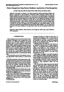
1. Introduction Tree search problems are very common in the pattern recognition field. For example, address recognition is usually carried out from a higher hierarchy like city names, narrowing down a lower hierarchy like street names, since address database is represented in a tree structure. Srihari first recognizes ZIP codes and primary numbers, and dynamically generates the street name lexicon [5]. Akiyama et al. first recognize higher level elements like city names and then narrow down lower level elements like street names [1]. In speech recognition, lexicon is often represented in a tree structure, by combining words sharing first some characters [3]. Search speed is accelerated thereby. Some face recognition algorithms first detect a face using a face detector, and recognize it afterwards [7]. This function can be seen as a two-stage tree structure, consisting of face detection process and face recognition process. More generally, in pattern recognition fast detectors/classifiers are often used in preprocess in order to narrow down the search area. In this paper, it is referred to as “hierarchical pattern recognition.” Beam search [3] was often employed for the search in those pattern recognition problems. Beam search needs a control on the pruning level according to the time limit. Recognition rate falls greatly when time limit varies for each data, since pruning level control is difficult in those cases. Best-first search [4] is a candidate for solving this difficulty. Best-first search is resistant to changing time limit, 978-0-7695-3725-2/09 $25.00 © 2009 IEEE DOI 10.1109/ICDAR.2009.231
street # 1A 1B 1001 1002 1 501 502 505
2. Relationship between pattern recognition and search Pattern recognition tasks often involve search. In this section, we illustrate the relationship between pattern recognition and search. First, let us take a look at an example of address recognition. In address recognition tasks you must solve a search problem, since address data are usually represented in tree structure. Fig.1 shows an example of an address database. The first, second and third layer correspond to city, street name and street number respectively. Fig.2(a) shows an ex461
Mr. ICDAR2009 CHIYODA 1002
g d
123-0011
(a)
f
e (b)
street
c, BUNKYO C d, BUNKYO
A
a, TOKYO
c, CHIYODA d, CHIYODA
B
c, TOKYO
g , BUNKYO
f, 1A f, 1B e, 1001 e, 1002 f, 1001 f, 1002 h, 1A h, 1B
C
D
E
FGH
street #
e, 1A e, 1B
B
Figure 4. The search tree for face detection and recognition
Figure 2. a: a mail image, b: word hypotheses city
I
face recognition
b
a
A
fine face detection
h
c
T OK Y O C I T Y JAPAN
coarse face detection
j
i
D E
C
2 2
D
A
1 1
2 2
E
6 6 6 3 3 3
B 2 2
F
2 2
3 3 3
4
4
1 1
4
4 5 5 5
3 3 3
Figure 5. An illustration of the search process described as a problem of searching the optimal terminal node in a tree, although there are some differences. Fast search algorithm for a tree structure is necessary in these problems, since there are quite a lot of terminal nodes.
Figure 3. The search tree for address recognition ample of a written address. Fig.2(b) shows word hypotheses derived from it. A word recognition module outputs a “score” for each combination of a word hypothesis and a word in the address database. A “score” may be a likelihood if you use an HMM, or it may be an averaged similarity of some character recognition processes, if you use a “segmentation & character recognition” approach. Fig.3 shows an example of a search tree. Each node in the search tree (white circle) corresponds to a combination of a word in the address database and a word hypothesis. Desirably, exhaustive matching may be performed, however it is extremely time consuming. Therefore, there arises a need for an effective search algorithm. Next let us take a look at a problem of detection of a face from an image and identification of the person by the face, as an example of hierarchical pattern recognition. The first step is the detection of a face by using a fast and light face detector on a lower resolution image. The detector is operated on every position and scale. The next step is the detection of a face by using a finer face detector on a higher resolution image. The detector is operated only on the possible position and scale narrowed down by the first step. The third step is the person identification by face on the same resolution image as the second step. The classifier is operated only on the possible position and scale narrowed down by the second step for all the registered persons. Fig.4 shows the search tree of this example. Each node in the search tree corresponds to a combination of the position in the image, scale and the person in the registration list for which the detector/classifier is operated. The position and scale of the node A in the lower resolution corresponds to the nodes B-E in the higher resolution. Nodes F-H stand for each registered person in the same position and scale as the node C. The above-mentioned two examples can commonly be
3. Search algorithms In this section, three search algorithms are described: beam search, best-first search and A* search. Their merits and demerits are discussed.
3.1. Beam search Beam search is a variation of breadth-first search algorithm in which pruning is done as the depth is increased 1 . N-best pruning or threshold pruning is done according to the evaluation value of each node. Circled numbers in Fig.5 stand for the order of nodes to be processed. B is pruned in step 1, so are C and E in step 2. Beam search have been widely used in the pattern recognition field. Conventional address recognition approach [5, 1] and hierarchical pattern recognition can be seen as beam search, since pruning is done as the depth is increased. The disadvantage of beam search is the difficulty and sometimes impossibility of controlling the pruning level. Excessive pruning leads to the fall of recognition rate, since the path containing the true answer can be eliminated. On the other hand, insufficient pruning leads to an increase in computation time, since too many nodes need to be processed. Recognition rate also drops when computation time is limited, since the search process cannot reach the terminal nodes. For these reasons, a fine tuning of the pruning level beforehand is necessary to maximize the recognition rate. However, the fine tuning is difficult when time limit varies for each data and is unknown before the search starts, leading to a low recognition rate. Above-mentioned cases 1 In the following, the term “beam search” is used in the meaning explained in this section, although it is used in some different ways.
462
term “admissible” means that the estimated value h satisfies h ≥ v. It is proven that the terminal node with the maximum evaluation value can be reached without full search if the evaluation function is admissible [4]. The problems of best-first search pointed out in section 3.2 can be resolved if you can design a good heuristic function. In speech recognition, an effective A* search is attained by designing a good heuristic function [3]. However, the problems that can be solved by this method is limited, since each problem needs a different heuristic function. An effective search cannot be attained when the estimation is inaccurate, even if a heuristic function is designed.
are not infrequent. Imagine a pattern recognition process, where the computation time consumed by the process prior to the search process varies. In those cases, the time given for the search for each data varies even if a constant time is given for the whole process. In address recognition, the time limit varies much, since there are lots of processes prior to search. Also difficulty of pruning level tuning arises in those cases when each node needs non-constant processing time. In address recognition, time consumption in each node usually varies, due to non-constant word length etc.
3.2. Best-first search
4. Bayesian best-first search
Best-first search is the technique of always expanding the node of the maximum evaluation value 2 3 . The search algorithm processes the nodes not always in the order of the depth. The node with the highest evaluation value is to be processed irrelevant to the depth. Italic number (1,2,3,...) next to the white circle in Fig.5 stand for the order of nodes to be processed. The search terminates by time limit in step 6, after reaching a terminal node in step 3 and continuing while there is still time. The merit of the best first search is the automatic control of pruning level. The method can get the result even when the time limit is very short, since the search reaches the terminal nodes early on in high rate. In the case of the longer time limit, the probability of getting the correct result is higher, since the search can reach more terminal nodes. This helps avoiding significant drop of recognition rate as in beam search, under the condition of the time limit varying by data. The main issue to realize this algorithm is the requirement of the evaluation value of the nodes comparable in arbitrary (different) depth. In beam search, each score computed as processing nodes can be directly used as the evaluation value, since they only have to be compared in the same depth level in the search. You can use the score of word recognition module for address recognition, that of face detector for face recognition respectively. This is not the case in best-first search. For example in Fig.3, you also have to take into account the score of the word recognition module for “a,TOKYO” (node A), together with that of “c,TOKYO” and “d,BUNKYO”, when you compare the node B and C. In the another example of Fig.4, you cannot compare the score of A and I, since the type of detectors for the two are different.
In this section, we propose Bayesian Best-first Search (BB Search), where a posteriori probability is used as the evaluation value in best-first search. Bayes’ decision rule is employed in BB search for comparing the evaluation values of nodes in different depth. Consider a non-terminal node equivalent to a combination of all its subnodes. For example in Fig.3, the event D is defied as “TOKYO is written in a, BUNKYO in c and 1A in e.” The event E is defined as “TOKYO is written in a, BUNKYO in c and 1B in e.” The event C is defined as “TOKYO is written in a, BUNKYO in c.” Assume that either 1A or 1B must be written in e whenever TOKYO is written in a and BUNKYO is written in c. In that case, event C is considered as (equivalent to) the combination of D and E. In Fig.4, event C is defined as “a face is in the specified position and size.” Event F(G,H) is defined as “the face of person 1(2,3) is in the specified position and size.” If only the faces of the registered three people appear in the image, event C is the combination of F, G and H. In the above formulation, each step in the search can be seen as the multi-class classification. For example in Fig.5, the next task is to choose the best node among B-F, if you are in the step 2. To solve the multi-class classification problem, using the Bayes’ decision rule is the best solution. This is the reason to use a posteriori probability for evaluation value in search.
5. Calculation of a posteriori probability In this section, we propose a way of calculating a posteriori probability. Examples where the output of the word recognition module is general score, a posteriori probability are described in section 5.1, 5.2 respectively for address recognition. A case of hierarchical pattern recognition like the face recognition is described in section 5.3. They can be treated in the same manner, although the meaning of the symbols are not always the same.
3.3. A* search A* search is a kind of best-first search which uses “admissible heuristic function” as the evaluation function. A “heuristic function” is a function which estimates the evaluation value v as the search reaches the terminal node. The 2 “Best-first search” is also used in some different meanings. In this paper, it is used as explained in this section, The interpretation is rather broad, which includes A* search. 3 Here, we deal with the case of expanding the nodes with the maximum evaluation values. The case of expanding the minimum ones are the same when you invert sign.
5.1. The case of general scores Let us denote the nodes by ni , i = 1, 2, .... Let the scores of the word recognition module be xi , respectively 463
n1 x1 n4 x4
n3 x3 n7
n2 x2
n8
n9 x9
n5
is written in word hypothesis c. It can be calculated from the distribution of the matching score of the correct words. The distribution can be obtained using training data. Alternatively, you may provide the distribution for each word length, if distributions vary greatly. You can also provide the distribution for each word, if enough training data is available. P (xj ) is the probability of the matching score being xj unconditionally. It can be calculated from the distribution of the matching score of any word hypotheses and words, whether they are correct or not. P (ni ) is a priori probability. You may assume P (ni ) of terminal nodes to be all equal, or estimate them by the frequency of addresses. P (ni ) of the parent node can be calculated by summing up all P (ni ) of its child nodes.
n6
n11 x11
n10 x10
Figure 6. An illustration of notation 4
. Let us denote collectively by X the scores for all the nodes already processed. For example in Fig.6, X = (x1 , x2 , x3 , x4 , x9 , x10 , x11 ) where the filled circles stand for processed nodes. A posteriori probability P (ni |X) is as follows: P (ni |X) =
P (X|ni )P (ni ) P (X) {∏
5.2. Cases when the score per se is a posteriori probability
} etc nj ∈Ui P (xj |ni ) P (Xi |ni ) {∏ } (2) etc nj ∈Ui P (xj ) P (Xi )
≈ P (ni ) ≈ P (ni )
(1)
∏ nj ∈Ui
P (xj |nj ) P (xj )
As to an HMM, a posteriori probability can be calculated as described later by using Bayes’ theorem, since the score of the word recognition module is a likelihood. Hamamura et al. propose a calculation method of a posteriori probability, for those algorithms not employing an HMM [2]. A method to calculate the a posteriori probability of nodes for these cases is described below. Let us use the same definition for ni , Ui as in section 5.1. Let hi be the word hypothesis corresponding to the node ni (e.g. h2 = h3 = c in Fig.3, when n2 = B, n3 = C). Let xi be the information used by the word recognition module while recognizing the word hypothesis hi . For example, xi is the feature vector sequence in an HMM approach, and collective recognition result of all the character hypotheses in hi in a segmentation & character recognition approach [2]. Let X be the collective information of all the word hypotheses. Let Xetc be the collective information of i the word hypotheses not corresponding to any of the nodes included in Ui . For example in Fig.3, U4 = {n1 , n3 , n4 } when n1 =A, n3 =C, n4 =D. In that case, word hypotheses of the nodes belonging to U4 are a, c, e. Therefore, Xetc 4 is the collective information of all the word hypotheses except a, c, e, that is b, d, f , g, h, i, j. Let wi be the word corresponding to node ni (e.g. w2=“TOKYO” when n2=B). The score (a posteriori probability) of word recognition module can be described as P (wi |xi ). According to the above definitions, the a posteriori probability P (ni |X), as an evaluation value for search, can be calculated with exactly the same equation as Eq.(1) (3), formally. However, the approximation P (Xetc i |ni ) ≈ P (Xetc i ) in Eq.(3) has a different meaning in this case. Here, the approximation is virtually an equation since Xetc i and ni share no word hypotheses. P (xj |nj ) P (xj ) in Eq.(3) is calculated as follows:
(3)
In Eq.(1), Bayes’ theorem was used. In Eq.(2), Ui is the set of ancestor nodes of ni and ni itself (e.g. U9 = {n1 , n4 , n9 } in Fig.6). Xetc is the collective denotation of i the scores for all the processed nodes not included in Ui (e.g. Xetc 9 = (x2 , x3 , x10 , x11 )). In Eq.(2), P (X|ni ) and P (X) are decomposed into products, by the assumption that the scores xi are independent to each other. This is a rough but useful approximation. In Eq.(3), we made two approximations. The first one is based on the assumption that the event probability of Xetc is unaffected by the event that ni is the correct one i or not. In the example of B and C in Fig.3, it means that the matching score of the word hypothesis c and “TOKYO” is unaffected by the event if “BUNKYO” is actually written in c. The assumption seems feasible, since the score becomes high only when “TOKYO” is actually written in c, while it generally becomes low when it is not. By this etc approximation, P (Xetc i |ni )≈P (Xi ) holds and the fraction is reduced. The second approximation is that the event probability of xj is unaffected by the event which subnodes of nj is the correct one. In the example of Fig.3, let xj be the score corresponding to C, the matching score of word hypothesis c and the word “BUNKYO”. In that case, the above approximation means that the probability of xj does not depend on whether the correct result is D or E, hence P (xj |D) ≈ P (xj |E) ≈ P (xj |C). This is practically an equality, rather than an approximation. Using this, P (xj |ni ) ≈ P (xj |nj ) (∀j, nj ∈ Ui ) in Eq.(2). The A posteriori probability of each node can be calculated using Eq.(3). P (xj |nj ) and P (xj ) can be calculated beforehand using training data. For example, at C in Fig.3, P (xj |nj ) is the probability of the matching score of c and “BUNKYO” being xj on the condition that “BUNKYO”
P (xj |nj ) P (xj |wj ) P (wj |xj ) ≈ = P (xj ) P (xj ) P (wj )
(4)
The first approximation is based on the assumption that a parent node does not affect its subnodes. For example in
4 We treat x as vectors for convenience, although actually they are i scalars.
464
recognition rate [%]
50
Figure 7. Examples of the address region Fig.3, it means that the word recognition result of node C is unaffected by the event if “TOKYO” is actually written in word hypothesis a. The second transformation is based on Bayes’ theorem. P (wj |xj ) in Eq.(4) is the score of word recognition module per se. You may assume P (wj ), an a priori probability of wj to be all equal, or you may estimate them by training data. You may also use Eq.(4) in an HMM approach if you can anyhow obtain P (xj ), since the likelihood, the score in an HMM approach is identical to P (xj |wj ).
40 30 20 10 0 1
2
5
10
20
50
100
BB
Figure 8. Comparison of the recognition rates
7. Conclusion In this paper, we proposed a search algorithm Bayesian Best-First Search (BB Search) suitable for pattern recognition. We pointed out disadvantages of beam search in pattern recognition, suggesting the solution by using bestfirst search. Next we employed Bayes’ decision rule for comparing nodes in different depth which is needed in bestfirst search. We further presented a derivation method of a posteriori probability. We demonstrated that BB search surpasses beam search by 12.4% in recognition rate, in the address recognition experiment using real postal images. For future work, we plan experiments other than address recognition.
5.3. Hierarchical pattern recognition The same technique as described in section 5.1 can be applied to hierarchical pattern recognition like the face recognition illustrated in Fig.4. A posteriori probability can be calculated using Eq.(3), by replacing the definition of xi in section 5.1 by the score of detector/classifier of node ni . The decomposition of the denominator into products in Eq.(2) may lead to a significant error. Since a lot of data can easily be collected for calculating P (xj ), one way to get around this problem is leaving some of the joint probability not decomposed into products.
Acknowledgments 6. Experiments We would like to thank Dr. Toshio Sato and Prof. Shigeki Sagayama who gave us helpful advices.
We conducted an address recognition simulation using 171 real European postal images to compare the BB search and beam search. Fig.7 shows examples of the address region of the postal image. Addressee is hidden for privacy protection. The address database is in a three level hierarchy. The three levels are city names, street names, street numbers, consisting of 1646, 345562, 2566421 data, respectively. Images without the correct database entry were omitted in advance. We employed the word recognition method we proposed in [2] with some modification for calculation during search. This method employs segmentation & character recognition approach, and outputs the a posteriori probability as the matching score. We used the structural approach for character segmentation. We employed a subspace method [6] for character recognition. We used N-best pruning for beam search under various N values. Fig.8 illustrates the recognition rates of beam search and BB search. In the x-axis, figures stand for the pruning limit N in the beam search and “BB” stands for BB search. In beam search, N = 5 gives the highest recognition rate. Lower rate in N5 is due to time out. The recognition rate of BB search surpasses the highest rate of beam search with N =5 by 12.4%. The result shows the advantage of BB search in the fluctuating time limit.
References [1] T. Akiyama, D. Nishiwaki, E. Ishidera, K. Kondoh, M. Hayashi, and T. Yamauchi. Alphabetical handwritten address recognition method allowing for no postal code and omission of several address elements. Technical Report of IEICE, PRMU2002-244:7–12, Mar. 2003 (in Japanese). [2] T. Hamamura, T. Akagi, and B. Irie. An analytic word recognition algorithm using a posteriori probability. Proc. 9th ICDAR, 2:669–673, 2007. [3] X. Huang, A. Acero, and H.-W. Hon. Spoken Language Processing: A Guide to Theory, Algorithm and System Development. Prentice Hall, 2001. [4] S. J. Russell and P. Norvig. Artificial Intelligence: A Modern Approach. Prentice Hall, 2002. [5] S. N. Srihari. Handwritten address interpretation: A task of many pattern recognition problems. Int’l J. Pattern Recognition and Artificial Intelligence, 14(5):663–674, 2000. [6] S. Watanabe and N. Pakvasa. Subspace method of pattern recognition. Proc. 1st. IJCPR, pages 25–32, 1973. [7] O. Yamaguchi and K. Fukui. “smartface” – a robust face recognition system under varying facial pose and expression. IEICE, J84-D-II(6):1045–1052, 2001 (in Japanese).
465