Bayesian decision feedback: equaliser for ... - Semantic Scholar

Bayesian decision feedback equaliser for overcoming co-channel interference S. Chen SMcLaughlin B.MuIgrew RM.Grant

In&.xing terms: Co-channel interference, Bayesian decision feedback equuliser

Abstract: The authors derive a Bayesian decision feedback equaliser which incorporates co-channcl interference compensation. By exploiting the structure of co-channel interfering signals, the proposed Bayesian decision feedback equaliser is able to distinguish an interfering signal from white noise and utilises this information to improve performance. Adaptive implementation of this Bayesian decision feedback equaliser includes identifying the channel model using the least mean square algorithm and estimating the co-channel states by means of an unsupervised clustering scheme. Simulation involving a binary signal constellation is used to compare both the theoretical and adaptive performance of this Bayesian decision feedback equaliser with those of the maximum likelihood sequence estimator. The results obtained indicate that, in the presence of severe co-channel interference, the Bayesian decision feedback equaliser employing the proposed simple scheme to compensate cochannel interference can outperform the maximum likelihood sequence estimator that only treats co-channel interference as an additional coloured noise.

1

Introduction

Adaptive equalisers for combating channel intersymbol interference (ISI) and noise can be classified into two categories, namely sequence estimation and symbol decision equalisers. The optimal solution for the class of sequence estimation equalisers is the maximum likelihood sequence estimator (MLSE) [I]. The MLSE provides the lowest error rate att,ainable for any equaliser when the channel is known but is computationally very expensive. A widely used symbol decision equaliser is the conventional decision feedback equaliser (DFE) [2] 0IEE, 1996 IEE Proceedings online no. 19960612 Paper first received 7th July 1995 and in revised form 25th March 1996 S. Chen is with the Department of Elecl.rical and Electronic Engineering, University of Portsmouth, Anglesea Building, Portsmouth PO1 3DJ, UK S. McLaughlin, B. Mulgrew and P.M. Grant are with the Department of Electrical Engineering, University of Edinburgh, King’s Buildings, Edinburgh EH9 3JL, UK IEE Proc.-Commun., Vol. 143, No. 4, Augu:it 1996

which has a very low computational complexity. The conventional DFE, however, does not achieve the full performance potential o f the symbol decision DFE structure, and the optimal symbol decision DFE is known to be the Bayesian DFE [3]. In the previous study [3-51, we have compared the Bayesian DFE with the conventional DFE and the MLSE extensively. In terms of computational requirements, the adaptive Bayesian DFE is more complex than the conventional DFE but is less complex than the adaptive MLSE. The adaptive MLSE requires sophisticated processing capability while the implementation o f the Bayesian DFE is relatively straightforward. For stationary channels, the performance of the adaptive Bayesian DFE is much better than the conventional adaptive DFE but is inferior to that of the adaptive MLSE. The adaptive Bayesian DFE however has significant advantages over the adaptive ML!SE for rapidly time-varying channels. Extensive simulation results have demonstrated that the adaptive Bayesian DFE actually outperforms the adaptive MLSE in terms of error rate for severely fading channels. It has been suggested that the adaptive MLSE accumulates tracking errors, which causes serious performance degradation [5]. Many communication systems, such as mobile cellular radio and dual polarised microwave radio channels, are impaired not only by channel IS1 but also by cochannel interference (CCI). It is well-known that an adaptive equaliser can usually do better against CCI than it can against the same level of noise [6]. However, in doing so, most of the equalisers can only treat CCI as an additional noise source and do not fully exploit the differences between the interfering signals and the noise. For example, a linear equaliser only exploits the spectral characteristics of the interference through its autocorrelations [6, 71. This is also the case for the conventional DFE studied in [8]. If both the channel and co-channels are known, it is possible to design the MLSE which takes into account both the IS1 and CCI. Such a full MLSE, although computationally very complex, will achieve the lowest possible error rate. The difficulty is that there is no practical way of obtaining accurate co-channel models needed. Unlike the case of channel identification.,there is generally no training signals available for supervised co-channel identification. Even if a means of identifying the co-channels can be developed, the estimate errors are expected to be large. The MLSE, being a sequence estimation method, is more likely to accumu219

late the co-channel estimation errors, causing serious performance degradation. In the blind equalisation setting, in theory it is possible to design a joint data detection and channelico-channels estimation based on the MLSE approach. Such an approach will certainly be computationally too expensive to implement. In practice, interfering signals are often treated as an additional coloured noise in the standard MLSE. The probability density function (PDF) of an interfering signal is quite different from that of the noise. An ideal equaliser should be capable of distinguishing the interfering signal from the noise. In a previous study [7],a Bayesian transversal equaliser was derived which can effectively exploit the differences between the CCI and the noise and uses this information to improve performance. The adaptive version of this Bayesian equaliser can be implemented easily. The present study extends this result to the DFE structure and incorporates CCI compensation into the Bayesian DFE derived previously for combatting IS1 and noise. It is shown that, in the presence of severe CCI, this Bayesian DFE has superior performance over the MLSE which only treats CCI as coloured noise. Adaptive implementation of this Bayesian DFE is then investigated. To effectively compensate for the CCI, the set of co-channel states are required. A simple unsupervised clustering algorithm is used to estimate these cochannel states.

The Bayesian D F E [3-51 was derived for complex valued multilevel signals. In the extension to include CCI, for notational simplicity and to highlight the basic concepts, s,(k),0 5 i 5 p , are assumed to be binary and to take values from the symbol set {dl)= +1, d2)= -1 }. The tap weights ulJ are therefore real valued. Application to complex valued A,(z) and multilevel symbol constellations are straightforward (as in the case of the Bayesian DFE for combating IS1 and noise) but the computational complexity will increase significantly. Let E[i2(k)]= 0," and E[u2(k)]= 0,". We define the signal to noise ratio (SNR) of the system as SNR= o!/oi, the signal to interference ratio (SIR) of the system as SIR = $/o;, and the signal to interference and noise ratio (SINR) of the system as SINR = o,'(o,' + o,"),respectively.

decision device

f iitering

@...l+J 1 j 2-1

Fig.2

Schematic of decision feedback equaliser

The structure of' the DFE considered in this study is depicted in Fig. 2. The equalisation process defined in Fig. 2 uses the information present in the observed channel output vector,

r(k) = [ ~ ( k ) . . . ~ ( ~ ~ - r n + i - ) ] * and the past detected symbol vector,

(3)

*

;b(k) = [So(k - d - 1). ' . So(k - d - n)] (4) to produce an estimate &(k - d) of so(k d).The integers d, rn and n are known as the decision delay, the feedforward order and the feedback order, respectively. Without the loss of generality, d = no - 1 is chosen to cover the entire channel dispersion Ao(z), m is related to d by m = d + 1 = no, and n is given by n = no + m d - 2 = ~ 1 0- 1 [3]. -

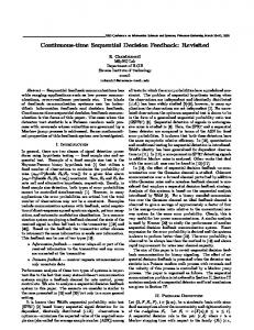
Fig. 1 Discrete-time model of communication system

-

The system model considered in this study is depicted in Fig. 1. This model [9] is widely used to represent communication systems in the presence of ISI, CCI and noise. The channel Ao(z) and the p interfering cochannels A,(z), l s i s p , are modelled by finite impulse response filters n2-1

A,(z) =

U , , ~ Z - ~0 ,

5i 5p

(1)

3=0

where n, and ai,,are the length and the tap weights of the ith impulse response, respectively. The transmitted data so(k) and the interfering data s,(k), 1 2 i 5 p , are independently identically distributed (iid) and they are mutually independent. The three components of the channel observation, ~ ( will be referred signal and the assumed to be E[e2(k)]= 0 .: 220

+

+

k=) ? ( k ) u ( k ) e ( k ) (2) to as the desired signal, the interfering noise, respectively. The noise e(k) is a Gaussian white noise with variance

2

Bayesian DFE in the absence of CCI

In the presence of the IS1 and noise, the optimal solution for the symbol decision structure of Fig. 2 is the Bayesian DFE [3-51. This Bayesian DFE is first summarised. This will naturally lead to the Bayesian solution in the presence of CCI. A new version of this Bayesian DFE is then presented which has certain practical advantages. Given the channel model Ao(z), the value of the noiseless channel output vector, f(k) = [ ? ( k ) .. . ? ( k - m + 1)]* (5) is specified by the symbol sequence s(k) = [s,@) sZ(k)lT, where Sf(k)

= [ s o @ ) .. . so(k - d ) ] T

]

(6) ~ b ( k= ) [sO(k - d - 1). . . sO(k - d - n)lT Under the assumption that the given feedback vector i s correct, that is, Ob(k)= sb(k), the state of i(k) is determined by sf(k). Since sf(k)has N, = 2d+1= 2" combinations, i ( k ) has N, states. Let N, sequences of sAk) be IEE Proc -Commun , Vol 143, No 4, August 1996

w,

= bS,3 ( k ). .Sf,j ( k 1 F j L Ns (7) Sf,3 The corresponding states of i(k), denoted as rJ, are given by: ’

r, = [F” F’][sfT,,,(k)G:(k)IT,

15j 5 N ,

(8)

where the m x (d + 1) matrix IT” has the form:

and the m x n matrix F’ has the form ... r o 0

0

ri = F ’ ’ S ~ ( k, )~, 1 5 J 5 N , (17) The Bayesian DFE consists of computing the decision variables: Np q2(k,ao)= exp(-llr’(k) - r;112/2a,2),1 5 i 5 2 (18)

1

3=1

and making the decision according to eqn. 14. This version of the Bayesian DFE realises the same optimal solution as the original one for the equalisation process defined in Fig. 2. It, however, has certain advantages over the original version. It removes the requirement of different Bayesian equalisers for different decision feedbacks, and has clear advantages in hardware implementation. Using the proposed translation, analysis of the Bayesian DFE can be redwed to one of studying an equivalent Bayesian equaliser ‘without decision feedback’. Schematic diagram of this alternative Bayesian DFE is depicted in Fig. 3.

1

The states of i(k) can be grouped into two subsets according to the value of so(k -- 9: ~ ( 2 )= {t(k) = ry)Iso(k - I-I) == s ( t ) } , 1 5 i 5 2 (11) Each R(j)contains iV,(j) = N,/2 = 2d states. is The PDF of r(k) conditioned on so(k d) =

r’(k)

~

r ’( k-2)

r ’ ( k-I)

r ‘ ( k-m +I )

1

N;tJ

pr(r(k)lso(k-d) = s ( ~ )=)

1a!i)pe(r(k)-rj), 1 I i I2

Bayesian equaliser

j=1

(12) where ri E R(j),aii)are a priori probabilities of ri, and p,(.) is the PDF of the noise vector e(k) = [e(k)... e(k m + l)]‘. Since all the channel states can be assumed to be equiprobable and the noise PDF is Gaussian, eqn. 12 leads to the Bayesian decision variables: Np

vi(k,ao)= 1 e x p ( - l / r ( k ) -r,jl12/2cz), 1 I i I 2 (13) j=1

Here a. = [ao,oao,l... ao,no.,]r i:; included in the expression to emphasise that the channel states are computed based on the given channel ;ao. The minimum error probability decision is defined by

-

3

Bayesian DFE in the presence of CCI

The Bayesian DFE can now readily be extended to cover CCI. The key to this extension is the fact that similar to the desired signal i ( k ) the interfering signal u(k) can only take some finite number of values. Without loss of generality, we will assume that only one CCI (p = 1) is present. The interfering signal u(k) then has Nu,$= 2nl scalar states {ui,1 5 j 5 Nu,s}.Therefore, the interfering signal vector, u ( k ) = [ u ( k ) . . u ( k - m l)IT (19) has Nu= 2n*+n1-1states. The set of these co-channel vector states is denoted as U = {uj, 1 5 j 5 N u } . In the presence of this CCI, the PDF o f r(k) conditioned on so(k d) = s(l)is

+

which provides the optimal solution for the equalisation structure o f Fig. 2 in the absence of CCI. For the above version of the Bayesian DFE originally derived in [3],a different set of the channel states is required at each sample k even when the channel a. is constant because the feedback vector $,(k) is different at different k. That is, different Bayesian equalisers are used for different decision feedbacks. Analysis and implementation of the Bayesian DFE becomes easier if the following space translation is made. Define: r’(k) = r(k) - F’Gb(k) (15) The elements of r’(k) can be computed recursively:

+

r’(k - 2 ) = z - l r ’ ( k - 2 1) - ao,,,_1S(k i = m - 1,.. . , 2 , 1 r’(k) = r ( k )

-

d - 1)

i

(16) In the new translated space, the channel states are given by IEE Pioc -Commun , Vol 143 N o 4 August 1996

~

N;jJ

p,(r(k)lso(k

-

d) = s ( 1 ) )=

N,,

x a ! ! p e ( r ( k ) - r j - ul) ,,=1 1=1

l 5 i 5 2 (20) where ri E R(j),ul E U and ay/ are a priori probabilities of rj + U/. Because all the rj + U1 are equiprobable and the noise PDF is Gaussian, the minimum error probability decision is achieved by computing the Bayesian decision variables: N.iZ1N,,

vt(k,ao) =

xexp(-IIr’(k) -ri

-

ul11~/2d

j=1 1x1

(21)

15252 and making the decision according to eqn. 14. 22 1

The computational complexity of the Bayesian DFE without CCI compensation is an order of N, [3, 51. The complexity of the Bayesian DFE with full CCI compensation is thus an order of N, x Nu. To reduce the complexity, an approximation of this full Bayesian DFE can be adopted which only approximates cochannel states. The approximation can easily be achieved due to the symmetric structure of co-channel states, and this will be illustrated using an example. Another reason for adopting the approximation is due to practical considerations. The scalar co-channel states U[ can only be estimated based on unsupervised learning. The resolution of unsupervised learning is limited, and it is not always possible to resolve all the co-channe1 states. In such a situation, it is natural to consider an approximation. Carrying out the approximation to an extreme and approximating the CCI as an additional noise, we obtain the Bayesian DFE with the decision variables: Np

Vz(k,a,) =

exp(-llr'(k)

-

r;1l2/2a2),1 5 i

I2

(22)

j=1

where rs2 = 0: + 0 .; This has the same form as the Bayesian DFE in the absence of CCI. h(0.50 +

Table 1: Scalar co-channel states for A,(z) 0 . 8 1 ~+' 0 . 3 1 ~ ~ ) NO.

(k)

SI

( k - 1 ) S, ( k - 2 )

SI

1

1

1

2

1

1

3 4

1 1

1 -1

-1 -1

5

-1

1

6

-1

1

7

-1

-1

8

-1

-1

1 -1 1 1 -1

21

.

'

U1

' ' '

2m-l

2m-l

2TT-l

U1 U2

' ' '

U2

'

No.

1

(k)

SI

(k-1)

ST

(k-2)

~1

1 1 1

1 1 1

1 1 -1

1 -1

U1

U1

U1

U1

U1

Y

1

U1

U2

U3

4 5

1

1

1

-1

-1

U1

U,

U,

1

1

U3

U5

1

1

1 -1

U?

6

-1 -1

U*

U,

U6

7

1 1

-1 -1

1 -1

U,

U4

U1

8

1 1

U,

U,

U,

9

1

1 -1

U5

U1

1

1 1

U3

10

-1 -1

U,

U,

U,

11

1 1

-1

-1

1 1

-1 -1

-1 -1

3

1 1 -1 -1 1 1 -1 -1

1.62 (h)

13

1.oo (1)

14

1 1

0.00 (1)

15

1

-1

-1

-1

16

1

-1

-1

-1

1 1

u3

1 -1

U4

U7

U5

U,

U,

U,

1 -1

U,

U8

U7

U,

U,

U*

1 -1

U5

U1

U1

U,

U,

U,

U5

Y

U3

U5

Y

U4

U3

U,

0.62 (1)

0.00 ( h )

18

-1 -1

-1 .oo ( h )

19

-1

1

1

-1

1

-1.62 (h)

20

-1

1

1

-1

-1

21

1 1

-1 -1

1 1

-1

U6

-1 -1

-1 -1

-1

U,

U,

U,

1 -1

U7

U5

U1

U7

U5

U,

1 1

1 1

1 1

1

24

-1

1

25 26

-1 -1

-1 -1

1 1

27

-1

-1

28

-1

-1

1 1

where the value of the parameter h dictates the SIR requirement. For example, h = 0.32 gives rise to a SIR = 1OdB. The set of the scalar co-channel states are listed in Table 1. The symmetric structure of the cochannel states is apparent in Table l. In general, this symmetric structure is expressed by the relationship:

29

-1

-1

-1

1

30

-1

-1

1

31

-1 -1

-1

-1

-1

32

-1

-1

-1

-1

+

+

}

1 5 1 5 Nu,s/2 (24) The set of the vector co-channel states U is obtained by expanding the scalar states. In this example, U contains 32 vector states as listed in Table 2. The rule to expand =

the set of the scalar co-channel states into the set of the vector co-channel states can be seen from Table 2. In general, in the table of the vector co-channel states, the last column (corresponding to u(k - m + 1)) is repeatedly filled with 20

QQ--Q 222

u3

-1

17

-1

Z0

U,

1 1 1

2

23

Z0

UN,>,' ' * UN,,,

(k-3) S, (k-4)

SI

22

UN,,,--l+l

'

Table 2: Vector co-channel states for A,(z) h(0.50 + 0 . 8 1 ~+' 0 . 3 1 ~ ~ )

We now use an example to illustrate the above discussion and to compare the theoretical performance of the Bayesian DFE with that of the MLSE which only treats the CCI as noise. The channel and the interfering co-channel are given by Ao(z)= 0.34 0.88x-l 0 . 3 4 ~ - ~ (23) Al(z)= X(0.50 0 . 8 1 ~ - ~0 . 3 1 ~ ~ ~ )

+

UN,,,uN,>,

..., and the first column (corresponding to u(k))is filled with

-1 -1

+

+ 2) is repeatedly

21

21

A A UlUl U 2 U 2 '

12

U,

-0.62 ( h )

-1

-- -

the column corresponding to u(k - m filled with

1 1 -1 -1

u6

u4

u6

-1 1

U,

U6

U,

U8

U7

U5

-1

1 -1

u7 '8

'8

'7

U,

U,

us

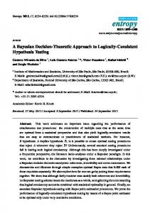
In this expansion, to obtain correctly the set of the vector co-channel states as shown in Table 2, we need to know the correct order of the scalar co-channel states as indicated in Table 1. The clustering algorithm described in the next Section can only identify the values of the scalar co-channel states and does not provide the information regarding their order. The order of the scalar co-channel states can be sorted out with the help of the state transition diagram. For the case of the eight scalar states, Fig. 4 depicts the state transition diagram. After the set of the eight scalar states has been obtained, by observing a sequence of states through time, their order can easily be arranged IEE Proc.-Commun., Vol. 143, No. 4, August 1996

according to the state transition diagram. The symmetric structure of the state transition diagram and the relationship of eqn. 24 helps to speed up this ordering process.

Table 4: SIR, SNR and SlNR values used to obtain the results of Figs. 6-8 Fig.

SIR 5dB

6

SNR

SlNR

2 - 28dB

0.3 - 5.0dB

7

10dB

2 - 25dB

1.4-

8

15dB

2-21dB

1.8- 14.0dB

9.8dB

-1 -!

-2-

v

Fig. 4

m. 0

State transition diagramfor case of eight scalar co-channel states

- .

01

2 -3-

Rearrange the eight scalar co-channel states of Table 1 into (1.62X,1.00X,0.62X,0.00~,-0.00X,-0.62X,-1.00X,-1.62X)

(25) We may approximate (1.621, 1.001) by its mean 1.311 and (0.621, 0.OOh) by 0.311,. This results in four approximated scalar co-channel states: (1.31X,0.31X, -0.31A, -1.31X) (26 1 The number of resulting approximated vector co-channe1 states is 16. This approximation may also be viewed from a different angle. The order of the co-channel is n1 = 3. Suppose that we only have an approximated cochannel order n^, = 2. This will give us four scalar cochannel states, and each of these approximated states is the mean of a pair of the true states. These four approximated scalar co-channel states are listed in Table 3 in the correct ordering, and the state transition diagram for the case of the four states is shown in Fig. 5. The Bayesian DFE with decision variables described by eqn. 22 may be viewed as the result of choosing 6,= 0.

-51

0

4

5

I

10

I

I

I

20

15

25

i

30

S N R , dB

Fig.6 -+-

Theoreticalperformance for SIR

= 5dB

MLSE treating CCI as noise -0- Bayesian D F E with approximated CCI compensation (SI= 2 ) -xBayesian D F E with full CCI compensation (SI7 n l = 3) Bayesian D F E without CCI compensation (rfl = 0) is similar to -+-

,I

-1 -1

-

-2

-

[r

w m

0

-

01

-0 - 3 -

Table 3: Approximated scalar co-channel states assuming = 2 for Al(z) h(0.50 + 0 . 0 1 , ~+~0 . 3 1 ~ - ~ )

nl

1

1

1

2

1

-1

3

-1

4

-1

1 -1

1.31 ( h )

-5 1 0

-0.31 (1) 0.31 (h) -1.31 (h)

Fig.7 -0-

-+-

-0-x-

Fig.5

State transition diagram for case of four scalar co-channel states

IEE Proc.-Commun.. Vol. 143, Nu. 4, Au,qust 1996

I

5

I

1

I

10 15 20 SNR, d 6 Theoreticalperformancefor SIR = 1OdB

25

Bayesian D F E without CCI compensation (rf, = 0) MLSE treating CCI as noise Bayesian D F E with approximated CCI compensation (ril = 2) Bayesian D F E with full CCI compensation (rfl = nl = 3)

Figs. 6 to 8 plot the performance curves of the Bayesian DFE without CCI compensation (n^, = 0), the MLSE which treats CCI as noise, the Bayesian DFE with an approximated CCI compensation (Al = 2) and the Bayesian DFE with the full CCI compensation (GI - nl = 3 ) for three different SIR conditions respectively. Table 4 summarises the SIR, SNR and SINR values used to obtain the results shown in Figs. 6 to 8. The performance of the Bayesian DFEs were obtained with detected symbols being fed back. When the ( X I is negligible, the MLSE has superior performance over the Bayesian DFE, as can be seen from the results of Fig. 8. However, in the presence of severe CCI, the 223

Bayesian DFE with an effective compensation of the CCI can outperform the MLSE that only treats the CCI as noise, as clearly shown in Figs. 6 and 7. 0

I

I

I

I

1

where g, is an adaptive gain. Given the channel estimate go, it is straightforward to calculate the set of the channel states r? from eqn. 17. The equaliser does not have access to the interfering data {s,(k)} or its estimate, and supervised learning such as the NLMS algorithm is not applicable for identifying the co-channel states. In the previous study [7], the unsupervised K-means clustering algorithm [ 101 is used to estimate the co-channel states. The ti-means clustering algorithm is known to be sensitive to the initial positions of the cluster centres. Recently, an enhanced K-means clustering algorithm has been proposed [I 11, which overcomes this drawback. This enhanced ti-means clustering algorithm is optimal in the sense that the variances of every cluster are equal after convergence. This property is particularly relevant for the application to estimate co-channel states since all the cluster variances in this case should be equal. Using this enhanced K-means clustering algorithm, we propose the following procedure to estimate the cochannel states: (i) Compute the channel residual ,

-61

I

Fig.8 -+-

I

I

5

0

I

20

10 15 SNR,dB Theoreticalperfbrmancefor SIR = 15dB

no-1

Bayesian DFE without CCI compensation (f, = 0) MLSE treating CCI as noise Bayesian DFE with full CCI compensation (n", = nl = 3)

E(k) = r ( k ) -

E

&o,jSo(k - j

)

(28)

j=O

where go = [bo,o...80,no-r]r is the current channel estimate. (ii) Compute the cluster variance weighted squared distances between the residual ~ ( kand ) the scalar co-channe1 states ui(k 11, 1 5 I S G,5

G(k) = U l ( k - l)C/(k) =~ l (k l)(~(k) ~ l ( -k 1))2,1 5 1

5 fiu,s(29)

where I$,s = 2'l, 6,is an estimate of the co-channel order, vl(k - 1) is the current variance of the Ith cluster ) ul(k and 8. In this = 4, regardless case, it may be sufficient to choose of the true number of the scalar co-channel states. For the system defined in eqn. 23 with SIR = lOdB and SNR = 15dB, the combincd NLMS and clustering learning was used to estimate the channel model and the scalar co-channel states. The channel order was assumed to be known and only an estimated co-channe1 order vil = 2 was assumed to be available. This gave rise to the four scalar co-channel states. The gain of the NLMS algorithm was chosen to be g, = 0.08. The parameters of the clustering procedure were set to: a = 0.999, gu = 0.05 and ~ ~ ( = 0 )0.000001 for all 1. Fig. 9 depicts a typical set of the scalar co-channel state trajectories obtained, where the lines indicate the expected values.

-i

0.2

Fig. 9 algorithm

1

I

- 1

0

60 80 100 samples Trajectories of scalar co-channel states obtained using clustering

40

20

Lines indicate expected values

-1

I c

\ t i1

t -5

A

0

Fig. 10 -0-

5

15 20 SNR, dB Adaptiveperjormance for SIR := lOdB

10

25

30

Bayesian DFE without CCI compensation (6,= 0) MLSE treating CCI as noise Bayesian DFE with approximated CCI compensation (t, = 2)

IEE Pror -Con?mun, Vol. 143. N o 4, August 1996

For the same system (eqn. 23) with SIR = lOdB, Fig. 10 compares the adaptive performance of the Bayesian DFE without CCI compensation (Z1 = 0), the MLSE which only treats CCI as noise and the Bayesian DFE with an approximate CCI compensation (uil = 2). In the first two cases, the NLMS algorithm used 100 training pairs (channel observations and transmitted symbols) to identify the channel model. For the last case, in addition, the clustering algorithm used 100 channel observation samples to estimate the four scalar cochannel states. The adaptive performance of the Bayesian DFE with an approximate CCI compensation ir very close to its theoretical performance, and is significantly better than that of the MLSE without CCI compensation.

5

Conclusions

Adaptive equalisation in the presence of ISI, additive Gaussian white noise and CCI has been investigated. It has been shown that, by exploiting the nature of interfering signals, the Bayesian DFE is capable of clistinguishing an interfering signal from the noise. Simulation results have demonstrated that, in the presence of severe CCI, the Bayesian DFE which incorporates CCI compensation can outperform the MLSE without CCI compensation. In theory, if an accurate knowledge of the channel and co-channels is known, the MLSE can be designed to take into account both the IS1 and CCI and hence outperforms the Bayesian DFE. In practice, however, adaptive implementation of such a MLSE is very difficult. Adaptive implemientation of the Bayesian DFE has been studied, and a. simple unsupervised clustering algorithm has been suggested to learn the co-channel states. This adaptive Bayesian DFE is particularly effective in compensating one or a few dominant interferences. A drawback of this adaptive scheme is that its computational complexity increases quickly as the size of the symbol constalletion increases. 6

References

1 FORNEY, G.D.: ‘Maximum-likelihood sequence estimation of digital sequences in the presence of intersymbol interference’, IEEE Trans., 1972, IT-18, (3), pp. 363-378 2 QURESHI, S.U.H.: ‘Adaptive equalization’, Proc. IEEE, 1985, 73, (9), pp. 1349-1387 3 CHEN, S., MULGREW, B., and MCLAUGHLIN, S.: ‘Adaptive Bayesian equaliser with decision feedback’, IEEE Trans., 1993, SP-41, (9), pp. 2918-2927 4 CHEN, S., MCLAUGHLIN, S., and MULGREW, B.: ‘Comdex-valued radial basis function network. Part 11: aoolication to higital communications channel equalisation’, E U R k I P Signal Proc. J., 1994, 36, pp. 175-188 5 CHEN. S., MCLAUGHLIN. S., MULGREW. B., and GRANT, P.M.: ‘Adaptive Bayesian decision feedback equaliser for dispersive mobile radio channels’, IEEE Trans., 1995, COM43, (5), pp. 1937-1946 6 PETERSEN, B.R., and FALCONER, D.D.: ‘Exploiting cyclostationary subscriber-loop interference by equalization’. Proceedings of GLOBECOM’90, San Diego, 1990, pp. 1156-1160 7 CHEN, S., and MULGREW, B.: ‘Overcoming co-channel interference using an adaptive radial basis function equaliser’, EURASIP Signal Proc. J . , 1992, 28, (l), pp. 91-107 8 FO, N.W.K., FALCONER, D.D., and SHEIKH, A.U.H.: Adaptive equalization for co-channel interference in a multipath fading environment’, IEEE Trans., 1995, COM-43, pp. 14411453 9 CAMPBELL, J.C., GIBBS, A.J., and SMITH, B.M.: ‘The cyclostationary nature of crosstalk interference from digital signals in multipair cable. Part I: fundamentals; Part 11: applications and further results’, IEEE Trans., 1983, COM-31, (S), pp. 629649 10 DUDA, R.O., and HART, P.E.: ‘Pattern classification and scene

analysis’ (John Wiley, New York, !973) 11 CHINRUNGRUENG, C., and SEQUIN, C.H.: ‘Optimal adaptive r-means algorithm with dynamic adjustment of learning rate’, IEEE Trans., 1995, “4,(l), pp. 157-169 22s