From Bayesian Decision-Makers to Bayesian Agents - Semantic Scholar

Book Title Book Editors IOS Press, 2003

1

From Bayesian Decision-Makers to Bayesian Agents Vaclav Šmídl, Jan Pˇrikryl Institute of Information Theory and Automation, Czech Academy of Sciences, Prague, Czech Republic AbstractBayesian approach to decision making is successfully applied in control theory for design of control strategy. However, it is based on on the assumption that a decision-maker is the only active part of the system. Relaxation of this assumption would allow us to build a framework for design of control strategy in multi-agent systems. In Bayesian framework, all information is represented by probability density functions. Therefore, communication and negotiation of Bayesian agents also needs to be facilitated by probabilities. Recent advances in Bayesian theory make formalization these tasks possible. In this paper, we bring the existing theoretic results together and show their relevance for multi-agent systems. The proposed approach is illustrated on the problem of feedback control of an urban traffic network. Keywords. Bayesian decision making, multi-agent systems, fully probabilistic design

1. Introduction In recent years, it becomes obvious that the traditional centralized approach to control of large systems has reached its limits. Decentralization of control and decision making is seen as future direction of research in both academia [13,7] and industry [14]. Many successful applications of so called holonic or multi-agent systems has been published. This paradigm presents a new challenge for designers of these systems, since the traditional methodologies of design became obsolete and no consistent replacement is available [14]. One possible solution of this problem is to extend the existing methodologies to accommodate the distributed setup. In control applications, we can see an agent as an entity consisting of two principal parts: (i) autonomous subsystem, which is responsible for agents ability to act according to its own aims and needs, and (ii) communication and negotiation subsystem, which is responsible for exchanging its knowledge with other agents and adjustment of its aims in order to cooperate and thus achieve better overall performance. The autonomous subsystem can be seen as a controller in the traditional sense, hence a number of methodologies for its design is readily available [10]. From this range of theories, we seek a methodology which is able to embrace not only the autonomous but also the communication and negotiation subsystem. The most promising candidate is the Bayesian theory of decision making, since (i) it is a consistent theory for dealing with uncertainty which is ever present in real environments [5], (ii) the task of agent communication and nego-

2

Enviroment Enviroment actions actions

data

actions data

Agent 1

data

Agent 2

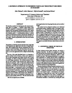
decision-maker communication Figure 1. Relation of Bayesian decision making and multi-agent systems.

tiation can be formalized as decision making problem, and (iii) it is successfully applied in controller design [18] and in design of advanced applications such as advising systems [19]. Traditionally, the decision-maker is assumed to be the only entity that intentionally influences the environment. It consists of a model of its environment, its individual aims, and a pre-determined strategy of decision making. The Bayesian decision-maker is designed by means of the Bayesian theory which results in probabilistic representation of all the components, i.e. model of environment, aims and strategy. An agent in multi-agent systems is known to influence only a part of the environment, i.e. its neighbourhood. The rest of the environment is modelled by other agents, as illustrated in Figure 1. In order to obtain relevant information from distant parts of the environment, an agent relies on communication with other agents in its neighbourhood. If the agents are able to exchange their aims and take them into account, they can cooperate and improve the overall performance of the system. The challenge for Bayesian decision making theory is to formalize communication and negotiation as operations on probability distributions. It was shown that the technique of fully probabilistic design (FPD) [17] reduces the task of agent cooperation into reporting and merging of probability density functions [1]. In this paper, we review Bayesian decision making in Section 2, and define the Bayesian decision-maker in Section 3. In Section 4, we bring together the latest achievements in application of Bayesian theory to multi-agent systems. The theory is applied to a practical problem of urban traffic control in Section 5. 2. Bayesian Decision Making Bayesian decision making (DM) is based on the following principle [5]: Incomplete knowledge and randomness have the same operational consequences for decision making. Therefore, all unknown quantities are treated as random variables and formulation of the problem and its solution are firmly based within the framework of probability calculus. This task of decision making can be decomposed into the following sub-tasks. Model Parametrization: Each agent must have its own model of its neighbourhood, i.e. part of the environment. Uncertainty in the model is described by parametrized probability density functions.

3

Enviroment actions ut

data yt

internal variables Θt observed data dt

decision-maker Figure 2. Basic decision making scenario.

Learning: Reduces uncertainty in the model of the neighbourhood, using the observed data. In practical terms, parameters of the model are inferred. Strategy Design: Choose the rule for generating decisions using the parametrized model and given aims. These tasks will be now described in detail. 2.1. Model Parametrization The basic scenario of decision making is illustrated in Figure 2. Here, dt denotes all 0 observable quantities on the environment, i.e. data, yt , and actions, ut , dt = [yt0 , u0t ] . Θt is an unknown parameter of the model of the environment. In Bayesian framework, the closed loop—i.e. the environment and the decision-maker—is described by the following probability density function: f (d (t) , Θ (t)) = t Y

f (yτ |uτ , d (τ − 1) , Θτ ) f (Θτ |uτ , d (τ − 1) , Θτ −1 ) f (uτ |d (τ − 1)) . (1)

τ =1

Here, f (·) denotes probability density function (pdf) of its argument. d (t) denotes the observation history d (t) = [d1 , . . . , dt ]. The model represents the whole trajectory of the system, including inputs uτ which can be influenced by the decision-maker. The chosen order of conditioning distinguishes the following important pdfs: observation model f (yt |ut , d(t − 1), Θt ) , which models dependency of the observed data on past data d (t − 1) = [d1 , . . . , dt−1 ], model parameters Θt and actions ut . internal model f (Θt |ut , d(t − 1), Θt−1 ) , which models evolution of parameters of the model via data history d (t − 1), previous model parameters Θt−1 and the chosen actions ut . DM strategy f (ut |d (t − 1)), is a probabilistic description of the decision rule. 2.2. Learning via Bayesian filtering The task of learning is to infer posterior distribution of unknown parameters from the observed data, f (Θt |d (t)). This pdf can be computed recursively as follows:

4

Z f (Θt |ut , d (t − 1)) =

f (Θt |ut , d (t − 1) , Θt−1 ) f (Θt−1 |d (t − 1)) dΘt−1(,2)

f (yt |ut , d (t − 1) , Θt ) f (Θt |ut , d (t − 1)) , f (yt |ut , d (t − 1)) Z f (yt |ut , d (t − 1)) = f (yt |ut , d (t − 1) , Θt ) f (Θt |ut , d (t − 1)) dΘt . f (Θt |d (t)) ∝

(3) (4)

In general, evaluation of the above pdfs is a complicated task, which is often intractable and many approximate techniques must be used [9]. In this text, we are concerned with conceptual issues and we assume that all operation (2)–(4) are tractable. 2.3. Design of DM strategy In this Section, we review fully probabilistic design (FPD) of the DM strategy [17]. This approach is an alternative to the standard stochastic control design, which is formulated as minimization of an expected loss function with respect to decision making strategies [2,6]. The FPD starts with specification of the decision making aim in the form of ideal pdf of the closed loop. This ideal pdf—which is the key object of this approach—is constructed in the same form as (1) distinguished by superscript bI: f (d (t) , Θ (t)) →

bI

f (d (t) , Θ (t)) .

(5)

Similarly to (1), the ideal distribution is decomposed into ideal observation model, internal model, and ideal DM strategy. Recall, from Section 2.1, that model (1) contains the DM strategy, which can be freely chosen. Therefore, the optimal DM strategy can be found by functional optimization of the following loss function 






 L f (ut |d (t − 1)) , ˚ t = KL f d ˚ t ,Θ ˚ t || bIf d ˚ t ,Θ ˚ t , where KL (·, ·) denotes the Kullback-Leibler divergence between the current (learnt) and the ideal pdf [27], and ˚ t > t is the decision making horizon. The approach has the following special features. • The KL divergence to an ideal pdf forms a special type of loss function that can be simply tailored both to deterministic and stochastic features of the considered DM problem. • Minimum of the KL divergence—i.e. the optimal DM strategy—is found in closed form: f (ut |d (t − 1)) =

bI

f (ut |d(t − 1))

exp[−ω(ut , d(t − 1))] , γ(d(t − 1))

(6)

where ω (·) and γ (·) are integral functions of all involved pdfs (these are not presented for brevity, see [19] for details). The decisions are then generated using a simplified version of stochastic dynamic programming [4]. • Multiple-objective decision making can be easily achieved using multi-modal ideal distributions [21,12].

5

3. Bayesian decision-maker In practise, the task of adaptive decision making is typically solved in two stages [19]: (i) off-line, and (ii) on-line. The off-line stage is dedicated to design of the structure and fixed parameters (such as initial conditions) of the decision-maker. When the structure and fixed parameters are determined, the decision-maker operates autonomously in online mode, where it is able to adapt (by adjusting model parameters) to changes in the environment and improve its DM-strategy. Operation needed in both stages are described in this Section. 3.1. Off-line stage In this stage, it is necessary to determine structure of the model (1) and prior distribution of model parameters. These tasks are solved using archives of the observed data as follows. Model selection: if there is no physically justified model of the environment, this technique test many possible parametrization of the model, and selects one, which is best suited for the observed data. Typically, only a class of models that yields computationally tractable algorithms is examined. A key requirement of tractability is, that the learning operation (2) can be reduced into algebraic operations on finite-dimensional statistics. Elicitation of prior distributions: The expert knowledge which is not available in the form of pdfs must be converted (often approximately) into probabilistic terms. Moreover, if the available knowledge is not compatible with the chosen model, a suitable approximation (projection into the chosen class) must be found. If there are more sources of prior information available, these must be merged into a single pdf. This operation will be described in detail at the end of this Section. Design of DM strategy: When the model and ideal distributions are chosen, the optimal DM strategy is given in closed form by the FPD (Section 2). In special cases, the equation (6) can be parametrized by a finite-dimensional parameters, and the implied dynamic programming is reduced into algebraic operations on these parameters. These tasks are computationally demanding and thus they are traditionally solved offline, i.e. only once for all available data. This is acceptable, since all expert information is available a priori, and model of the environment is assumed to be constant. 3.2. On-line stage A typical adaptive decision-maker operates by recursive repetition of the following steps: 1. read: the observed data are read from the environment. All the necessary preprocessing and transformation of data is done in this step. 2. learn: the observed data are used to increase the knowledge about the environment, namely the sufficient statistics of the model parameters are updated. 3. adapt: the decision-maker use the improved knowledge of the system to improve its DM strategy. Specifically, parameters of the DM strategy are re-evaluated using the new sufficient statistics.

6

4. decide: the adapted DM strategy is used to choose an appropriate action. Recall, that the DM-strategy is a pdf. Hence, a realization from this pdf must be selected. Typically, the optimal decision is chosen as expected value of (6). 5. write: the chosen action is written into the environment. Similar to the first step, transformation of the results is done in this step. Note that due to computational constraints, all operations in this stage are defined on finite dimensional parameters or statistics. 3.3. Merging of pdfs For the task of prior elicitation, we need to define a new probabilistic operation for merging of information from many sources. The merging operation is defined as a mapping of two pdfs into one: merge f1 (Θt |d (t)) , f2 (Θt |d (t)) −→ f˜ (Θt |d (t)) ,

(7)

where f1 and f2 are the source pdfs, and the f˜ is the merged pdf. Many approaches are available, e.g. [16,15,19], with different assumptions and properties. Here, we review results of [24,23] since these have the following properties: (i) defined as optimization problems, with a reasonable loss function, (ii) their results are intuitively appealing and well interpretable, (iii) the optimum is reached for a class of pdfs which is uniquely defined, (iv) is applicable to both discrete and continuous distributions, and (v) algorithmic solutions are available. We distinguish two kinds of merging: direct: the source and the merged pdfs are defined on the same variables, such as (7), indirect: the source distributions are defined on the variable in condition of the merged pdf. These will be now described in detail. 3.3.1. Direct merging The task of direct merging can be defined as optimization problem where the optimized function, LM , is chosen as divergence between the source and the merged pdfs [23] as follows: LM (f ) = αKL (f2 ||f ) + (1 − α) KL (f1 ||f ) .

(8)

Here, KL (·, ·) denotes the Kullback-Leibler divergence, the weight α ∈ h0, 1i governs the level of importance of each source, and f is the optimized pdf. The merged pdf f˜ (d) is found by functional minimization of (8): f˜ = arg min LM (f ) . f

(9)

The optimum (9) for merging of distributions of the same variable, is found in the form of a probabilistic mixture of the source pdfs:

7

f˜ (d) = αf2 (d) + (1 − α) f1 (d) .

(10)

This solution is intuitively appealing and has been proposed using heuristic arguments [15]. Solution of the problem for multivariate distributions with various length of variables is more complicated, the result can not be found in closed form, however an iterative algorithm which asymptotically converge to the optimum is available [22]. This algorithms is feasible for discrete distributions. For continuous variables, complexity of the merged distribution grows with each iteration, and further approximations must be used. 3.3.2. Indirect Merging The operation of indirect merging is defined as follows: merge f1 (dt |d (t − 1)) , f2 (dt |d (t − 1)) , f (Θt |dt ) −→ f˜ (Θt |d (t)) .

(11)

This operation can be seen as generalization of the Bayes rule, since it reduces to Bayesian learning (3) if the sources, f1 and f2 , are empirical densities. Using (10) and generalized Bayesian estimation the problem can be solved as follows [24]:   Z f˜ (Θt |d (t)) ∝ f (Θt ) exp −n αf1 (dt |d (t − 1)) ln f (dt |Θt ) ddt ×  × exp −n



Z (1 − α) f2 (dt |d (t − 1)) ln f (dt |Θt ) ddt

Complexity of this operation is comparable to that of the Bayesian learning (3).

4. Bayesian Agents The Bayesian agent is an extended Bayesian decision-maker described in previous Section. The additional features are the ability and need of agents to communicate and cooperate. In the Bayesian framework, all knowledge is stored in pdfs. The challenge is to formalize communication and cooperation within the framework of probability calculus. In this Section, we propose a simple probabilistic model of negotiation. For clarity of explanation, we consider only two agents, A[1] and A[2] , where agent number is always in subscript in square brackets. Each agent has the following quantities Observed data dt : Naturally, each agent can observe different subset of variables, i.e. dt,[1] and dt,[2] , for A1 and A2 , respectively. The agents can exchange knowledge only in terms of variables that are common for both of them, i.e. dt,[1∩2] . Any communication is meaningful only with respect to this subset. Internal quantities Θt : We do not impose any structure of the environment model for the agents, hence, internal quantities Θt,[1] and Θt,[2] are in general disjoint sets.

Environment Model: f[1] = f d[1] (t) , Θ[1] (t) and f[2] = f d[2] (t) , Θ[2] (t) for each agent.

8



Ideal distributions: bIf[1] = bIf d[1] (t) , Θ[1] (t) and bIf[2] = bIf d[2] (t) , Θ[2] (t) for each agent. Negotiation weights: For the purpose of negotiation, we define a scalar quantity α2,[1] ∈ h0, 1i denoting the level of belief of agent A1 in information received from A2 . Analogically, α1,[2] is defined in A2 . 4.1. Communication The agents can communicate two kinds of information: (i) about the environment, and (ii) about their individual aims. In both cases, the information is stored in the form of pdfs, namely marginal distribution from the environment model for (i), and marginal distribution on ideal pdfs for (ii). The model of the environment (1) is fully determined by the observation model (Section 2.1) and parameter distribution (3), which is estimated from the observed data d(t). The easiest way how to exchange the information about the environment is to exchange the observed data.
The observed data can be seen as a special case of pdf, namely empirical pdf f d[2] (t) . Then, the task is formally identical with the task of indirect merging of pdf (11) as described in Section 3.3. The observed data from A2 are merged with the existing model of A1 using
merge f[1] , f d[2] (t) −→ f˜[1] . and the negotiation weight α2,[1] . This weight can be chosen constant or it can be negotiated with the neighbour. When the negotiation is finished, the merged pdf f˜[1] is then used as the new model of the environment. The ideal distributions can be communicated and merged in the same way, using direct merging (7). Note that merging of the ideal distributions influences the aim of the agent. The FPD procedure must be performed after each merge in order to recompute the DM strategy. Once again, the result is strongly influenced by the negotiation weights α. These weights can be determined by negotiation strategies. If the merging operation yields pdfs that are not compatible with the observation model (i.e. can not be reduced into algebraic form), the merged distribution must be projected into the compatible class, as illustrated in Figure 3. 4.2. Negotiation strategies We distinguish three basic strategies [20]: • selfish — a strategy where each agent freely chooses its own weights. Agent A1 accepts all information from its neighbour, but it refuse any attempts to change the weight α2,[1] that may be suggested by A2 . • hierarchical — a strategy where the agent have a fixed values of α2,[1] , however if the neighbour A2 is superordinate to A1 , it can assign the value of α2,[1] by communication. • cooperative — a strategy, where both participants have common aim (given by the user using ideal pdfs) to reach an agreement on the negotiation values, i.e. α2,[1] = α1,[2] .

9

A[1]

A[2] f[2]

f[1] 0

5

10

15

20

0

5

10

15

20

α2,[1] = 0.2 Merging mixture

0 5 Projection

0

5

10

15

10

15

20

20

Figure 3. Illustration of merging of two Gaussian distribution. The merged distribution is a mixture of Gaussians for which the operations of learning and design of DM strategy do not have a finite-dimensional parametrization. Thus, the merged distribution is projected into the class of single Gaussians.

4.3. On-line algorithm of Bayesian agents On-line operation of each Bayesian agent is an extension of the on-line steps of Bayesian decision-maker (Section 3). 1. read: the observed data are read from the system (environment). Possible communication (via pdf) from the neighbour is also received in this step. We assume that only one neighbour can communicate in one time step. 2. learn: the observed data are used to increase the knowledge about the system (environment). 2a. merge: if the communication from the neighbour contains information about the environment, the merge operation is called in order to merge it with the current knowledge. In case of communication of ideal distributions, the FPD procedure is run. Note that this step may be computationally expensive. 3. adapt: the decision-maker use the improved knowledge of the environment to improve its DM strategy. 4. decide: the adapted DM strategy is used to choose an appropriate action. In multiagent scenario, the tasks of communication and negotiation are also part of the decision making process. Therefore, in this step, decisions on communication (re-

10

quest communication, negotiate, refuse communication) and negotiation (propose new value of α1,[2] ) must be also made. 5. write: the chosen action is written into the system (environment). If the decision to communicate was made, a message to the neighbour is also written in this step. Note that acquisition of the observed data is synchronized with communication. In each time step, only one message from the neighbour is received, processed and answered. This allows seamless merging of knowledge from direct observations and from communication. If the periods of data sampling and communication differ, the smaller one is chosen as the period of one step of an agent.

5. Application in Traffic Control Urban surface transport networks are characterised by high density of streets and a large amount of junctions. In many cities these structures cannot easily accommodate the vast volume of traffic, which results in regular traffic congestions. Efficient traffic control mechanisms are sought that would provide for higher throughput of the urban transport network without changing its topology. Due to space constraints we cannot present the reader with full introduction to the principles of urban traffic control (UTC). We will just briefly outline terms that will be needed below. More thorough explanation of the UTC methodology exceeds the scope of this paper. Interested readers should refer to any of the existing monographs on this topic, e.g. [28,31]. In most cases, UTC is targeted on signalled intersections, where traffic is controlled by traffic signals. The sequence of traffic signal settings for an intersection is called a signal plan. A signal plan cycle typically consist of several stages, where one of the conflicting traffic flows has green and the others have to wait. The lengths of stages, the overall signal plan duration and other parameters are bounded by values reflecting either physical shape of the intersection or other (usually normatively given) rules. An intersection controller is an industrial micro-controller that attempts to select the order of stages and to modify stage lengths in such a way that a maximum possible throughput of the intersection is achieved. The ordering of stages may be influenced by public transport vehicles in order to minimise their waiting at an intersection. Intersection controllers are very often autonomous devices that do not react on traffic conditions at neighbouring intersections. However, in areas with high traffic intensity, intersection controllers may be mutually interconnected in a kind of hierarchical controller that attempts to optimize the throughput of the whole traffic network. Several interesting UTC approaches exist that attempt to solve the traffic control problem using feedback from different traffic detectors [25]. Many agent-based approaches have been implemented as well. For example: (i) agents for setting of the optimal signal plan cycle length [11], and (ii) for distributed coordination of signal plans. The latter are based on game theory [3,8] or Bayesian learning [29]. These applications often use approximate heuristics and long-time statistics to derive the optimal control strategy. Our proposal is to build the strategy adaptively in a collaborative agent-based environment. In the following text, agents are intersection controllers of some street network. The agents shall agree on the overall traffic signal setting that would minimise time spent by vehicles inside the controlled region and thus maximise the throughput of the network.

11

5.1. Model Papageorgiou [30] shows that the total time spent by a vehicle in a controlled microregion is strongly correlated to queue lengths at signalised intersections of this microregion. Hence, minimization of waiting queues results in faster vehicle transition and in higher throughput of the network. We start with a deterministic model describing the behaviour of the traffic at an intersection as a particle flow system [26]: Θt = AΘt−1 + But−1 + F yt = CΘt + G where  Θt =

ξt Ot



is a state vector holding information about waiting queue lengths ξt and detected input lane occupancies Ot , ut is an input variable which represents green settings for a signal plan cycle at this intersection. Matrix A defines transition from an old state to the new one. It is composed from information about waiting queue development, and mutual influence of queues at one lane on other lanes. Matrix B models throughput of the junction, and vector F is composed from the observed incoming traffic intensity. Output vector 

ηt yt = Ot0



contains information about outgoing traffic intensity ηt and output arm occupancies Ot0 . C is a matrix of coefficients transforming waiting queue data into outgoing traffic intensities and vector G models the influence of current incoming traffic and past queues on outgoing traffic. This model can be transcribed into the following probabilistic internal and observation models: f (Θt |Θt−1 , ut−1 ) = N (AΘt−1 + But−1 + F, Q) f (yt |Θt ) = N (CΘt + G, R)

(12) (13)

where N (µ, σ) is a Gaussian probability distribution and Q and R are allowed variances. The internal model (12) describes the probability distribution of queue lengths at an intersection at time t given the green settings ut−1 and incoming traffic data Θt−1 at time t − 1. The observation model (13) yields probability distribution of outgoing traffic intensity of the modelled junction at time t, given the queue pdf from the internal model. 5.2. Ideal distributions The global aim of the proposed UTC approach is to minimise waiting queues at every junction. As said in Section 4, agents attempt to reach this aim by exchanging their ideal pdfs, defined on their common data. In our case, agents share information about traffic

12

Junction agent #1

Junction agent #2

Junction agent message channel #3

Junction agent #4

output detector input detector

Figure 4. Simple urban traffic network with four controlled junctions and four agents.

intensity at particular intersection arms. Hence, the exchanged ideal pdfs specify wishes about intensity of outgoing and incoming traffic. We propose to model the ideal pdfs as follows: bI

f (ξt ) = tN (0, Vξ , h0, ξmax i) ,

(14)

bI

f (It |ξt ) = tN (I (ξt ) , VI , h0, Imax i) ,

(15)

bI

f (ηt |ξt ) = tN (ηmax , Vη , h0, ηmax i) .

(16)

Here, tN (0, U, h0, ξmax i) denotes a Gaussian distribution with mean value 0 and variance Vξ , truncated on the interval h0, ξmax i. ξmax denotes maximal allowed queue length. The ideal (14) favours minimal queue lengths value, since estimates f (ξt ) with lower mean value are closer to the ideal than those with larger mean value. The ideal pdf (15) models the agents wishes for input intensities coming from its neighbours. The requested mean value I (ξt ) is changing with the current traffic conditions. The variance VI expresses the “strength” of the request; higher VI allows higher deviation from ideal I (·) and leaves the agent more room for adapting to other requests. Imax is the maximum possible intensity at the arm (or lane) in concern. In order to communicate these wishes to the neighbours, they must be independent of the internal quantity ξt . This can be achieved by marginalization, i.e. bIf (It |ξt ) → bIf (It ). Note that output intensities of one intersection are input intensities of its neighbours,
will be i.e. ηt,[1] → It,[2] . Hence, the communicated ideals on input intensities f I t,[2]
merged with ideals on output intensities f ηt,[1] . 5.3. Control cycle The proposed control cycle of a single agent follows the decomposition from Section 4.3: 1. read: The agent reads observed data from the environment and checks for incoming communication from some neighbour.

13

2. learn: Observed data of the agent (measured traffic intensities) are used to increase its knowledge about current traffic conditions, namely pdfs of waiting queue lengths and unobserved intensities of traffic flow. 3. merge: If a message from some neighbour arrived, its pdf is merged with the agent’s pdfs — either with the current knowledge or with ideal pdfs. In the latter case, FPD procedure that evaluates Eq. (6) is called after the merge in order to reflect the change in ideal aims in the optimal DM strategy. 4. adapt: The agent uses the updated knowledge to adapts its DM strategy. Hence, the strategy can be changes in reaction to the changed traffic conditions or in reaction to the message from the neighbour. 5. decide: Based on the adapted strategy, the agent decides about its signal plan parameters for the next period. The signal values are typically taken as expected values of the adapted strategy pdf. Decisions whether and what to communicate with agent’s neighbour is also made in this moment. 6. write: The chosen signal plan is written to the intersection controller. Optionally, communication message is sent to the chosen neighbour.

6. Conclusion We have presented an application of the Bayesian decision making theory to the area of multi-agent systems. The presented methodology offers clear guidelines and concept of design of multi-agent systems. Since the Bayesian approach formalizes all available knowledge in the form of probability density functions, we had to formalize the key features of agents—i.e. communication and negotiation—using probability calculus. We have shown that the formalization can be achieved using techniques of fully probabilistic design and merging of pdfs. The work presented in this paper is a conceptual outline of the approach. In spite of the fact that the key techniques are available, many practical issues must be solved before it is ready for real application. The presented application in urban traffic control will be used as testing environment for further research and development of Bayesian agents. Acknowledgements ˇ 1ET 100 750 401 This work was supported by grants MŠMT 1M0572 (DAR) and AVCR (BADDYR).

References [1] J. Andrýsek, M. Kárný, and J. Kracík, editors. Multiple Participant Decision Making, Adelaide, May 2004. Advanced Knowledge International. [2] K.J. Astrom. Introduction to Stochastic Control. Academic Press, New York, 1970. [3] Ana L. C. Bazzan. A distributed approach for coordination of traffic signal agents. Autonomous Agents and Multi-Agent Systems, 10(1):131–164, January 2005. [4] R. Bellman. Introduction to the Mathematical Theory of Control Processes. Academic Press, New York, 1967. [5] J.O. Berger. Statistical Decision Theory and Bayesian Analysis. Springer-Verlag, New York, 1985.

14

[6] D.P. Bertsekas. Dynamic Programming and Optimal Control. Athena Scientific, Nashua, US, 2001. 2nd edition. [7] R. Caballero, T. Gomez, M. Luque, F. Miguel, and F. Ruiz. Hierarchical generation of pareto optimal solutions in large-scale multiobjective systems. Computers and operations research, 29(11):1537–1558, 2002. [8] Eduardo Camponogara and Werner Kraus Jr. Distributed learning agents in urban traffic control. In Fernando Moura Pires and Salvador Abreu, editors, Progress in Artificial Intelligence: Proceedings of the 11th Portuguese Conference on Artificial Intelligence (EPIA 2003), volume 2902 of Lecture Notes in Computer Science, pages 324–335, Beja, Portugal, December 2003. Springer-Verlag. [9] Z. Chen. Bayesian filtering: From Kalman filters to particle filters, and beyond. Technical report, Adaptive Syst. Lab., McMaster University, Hamilton, ON, Canada, 2003. [10] B. Tamer (ed.). Control Theory. IEEE Press, New York, 2001. [11] L. A. García and F. Toledo. An agent for providing the optimum cycle length value in urban traffic areas constrained by soft temporal deadlines. In L. Monostori, J. Váncza, and M. Ali, editors, Engineering of Intelligent Systems: 14th International Conference on Industrial and Engineering Applications of Artificial Intelligence and Expert Systems, IEA/AIE 2001, volume 2070 of Lecture Notes in Computer Science, pages 592–601, Budapest, Hungary, June 2001. Springer-Verlag. [12] T.V. Guy, J. Böhm, and M. Kárný. Multiobjective probabilistic mixture control. In IFAC, editor, IFAC World Congress, Preprints. IFAC, Prague, 2005. accepted. [13] Y.Y. Haimes and D. Li. Hierarchical multiobjective analysis for large scale systems: Review and current status. Automatica, 24(1):53–69, 1988. [14] K. H. Hall, R. J. Staron, and P. Vrba. Holonic and agent-based control. In Proceedings of the 16th IFAC Congress, 2005. [15] F.V. Jensen. Bayesian Networks and Decision Graphs. Springer-Verlag, New York, 2001. [16] R. Jiroušek. On experimental system for multidimensional model development MUDIN. Neural Network World, (5):513–520, 2003. [17] M. Kárný. Towards fully probabilistic control design. Automatica, 32(12):1719–1722, 1996. [18] M. Kárný. Tools for computer-aided design of adaptive controllers. IEE Proceedings — Control Theory and Applications, 150(6):642, 2003. [19] M. Kárný, J. Böhm, T. V. Guy, L. Jirsa, I. Nagy, P. Nedoma, and L. Tesaˇr. Optimized Bayesian Dynamic Advising: Theory and Algorithms. Springer, London, 2005. [20] M. Kárný and T.V. Guy. On dynamic decision-making scenarios with multiple participants. In J. Andrýsek, M. Kárný, and J. Kracík, editors, Multiple Participant Decision Making, pages 17–28, Adelaide, May 2004. Advanced Knowledge International. [21] M. Kárný and J. Kracík. A normative probabilistic design of a fair governmental decision strategy. Journal of Multi-Criteria Decision Analysis, 10:1–15, 2004. [22] J. Kracík. Composition of probability density functions - optimizing approach. Technical ˇ Praha, 2004. Report 2099, ÚTIA AV CR, [23] J. Kracík. On composition of probability density functions. In J. Andrýsek, M. Kárný, and J. Kracík, editors, Multiple Participant Decision Making, volume 9 of International Series on Advanced Intelligence, pages 113–121. Advanced Knowledge International, Adelaide, Australia, 2004. [24] J. Kracík and Kárný M. Merging of data knowledge in Bayesian estimation. In Proceedings of the Second International Conference on Informatics in Control, Automation and Robotics, pages 229–232, Barcelona, September 2005. [25] J. Kratochvílová and I. Nagy. Bibliographic Search for Optimization Methods of Signal ˇ Praha, 2003. Traffic Control. Technical Report 2081, ÚTIA AV CR, [26] J. Kratochvílová and I. Nagy. Traffic model of a microregion. In IFAC, editor, IFAC World Congress, Preprints. IFAC, Prague, 2005. submitted. [27] S. Kullback and R. Leibler. On information and sufficiency. Annals of Mathematical Statis-

15

tics, 22:79–87, 1951. [28] Michael Meyer and Eric J. Miller. Urban Transportation Planning. McGraw-Hill, 2 edition, December 2000. [29] Haitao Ou, Weidong Zhang, Wenjing Zhang, and Xiaoming Xu. Urban traffic multi-agent system based on rmm and bayesian learning. In Proceedings of the American Control Conference, Chicago, Illinois, June 2000. [30] M. Papageorgiou. Applications of Automatic Control Concepts to Traffic Flow Modeling and Control, volume 50 of Lecture Notes in Control and Information Sciences. Springer-Verlag, Berlin, 1983. [31] Roger P. Roess, Elena S. Prassas, and William R. McShane. Traffic Engineering. Prentice Hall, 3 edition, October 2003.