Bayesian Haplotype Inference via the Dirichlet Process∗ Eric P. Xing†‡
Michael I. Jordan§
Roded Sharan¶
Abstract The problem of inferring haplotypes from genotypes of single nucleotide polymorphisms (SNPs) is essential for the understanding of genetic variation within and among populations, with important applications to the genetic analysis of disease propensities and other complex traits. The problem can be formulated as a mixture model, where the mixture components correspond to the pool of haplotypes in the population. The size of this pool is unknown; indeed, knowing the size of the pool would correspond to knowing something significant about the genome and its history. Thus methods for fitting the genotype mixture must crucially address the problem of estimating a mixture with an unknown number of mixture components. In this paper we present a Bayesian approach to this problem based on a nonparametric prior known as the Dirichlet process. The model also incorporates a likelihood that captures statistical errors in the haplotype/genotype relationship trading off these errors against the size of the pool of haplotypes. We describe an algorithm based on Markov chain Monte Carlo for posterior inference in our model. The overall result is a flexible Bayesian method, referred to as DP-Haplotyper, that is reminiscent of parsimony methods in its preference for small haplotype pools. We further generalize the model to treat pedigree relationships (e.g., trios) between the population’s genotypes. We apply DP-Haplotyper to the analysis of both simulated and real genotype data, and compare to extant methods.
1
Introduction
The availability of a nearly complete human genome sequence makes it possible to begin to explore individual differences between DNA sequences on a genome-wide scale, and to search for associations of such genotypic variation with disease and other phenotypes [17]. The largest class of individual differences in DNA are the single nucleotide polymorphisms (SNPs). Millions of SNPs have been detected thus far out of an estimated total of ten million common SNPs [18]. A SNP commonly has two variants, or alleles, in the population, corresponding to two specific nucleotides chosen from {A, C, G, T }. A haplotype is a list of alleles at contiguous sites in a local region of a single chromosome. Assuming no recombination in this local region, a haplotype is inherited as a unit. Recall that for diploid organisms (such as humans) the chromosomes come in pairs. Thus two haplotypes go together to make up a genotype, which is the list of unordered pairs of alleles in a region. That is, a genotype is obtained from a pair of haplotypes by omitting the specification of the association of each allele with one of the two chromosomes—its phase. Common biological methods for assaying genotypes typically do not provide phase information; phase can be obtained at a considerably higher cost [16]. It is desirable to develop automatic methods for inferring haplotypes from genotypes and possibly other data sources (e.g., pedigrees). With a set of inferred haplotypes in hand, associations to disease can be explored. From the point of view of population genetics, the basic model underlying the haplotype inference problem is a finite mixture model. That is, letting H denote the set of all possible haplotypes associated with a given ∗A
preliminary version of this paper appeared in [20]. whom correspondence should be addressed. ‡ School of Computer Science, Carnegie Mellon University, Pittsburgh, PA 15213.
[email protected]. § Computer Science Division, Department of Statistics, University of California at Berkeley, Berkeley, CA 94720-1776.
[email protected]. ¶ School of Computer Science, Tel-Aviv University, Tel-Aviv 69978, Israel.
[email protected]. † To
1
region (a set of cardinality 2k in the case of binary polymorphisms, where k is the number of heterozygous SNPs), the probability of a genotype is given by: X p(g) = p(h1 , h2 )I(h1 ⊕ h2 = g) (1) h1 ,h2 ∈H
where I(h1 ⊕ h2 = g) is the indicator function of the event that haplotypes h1 and h2 are consistent with g. Under the assumption of Hardy-Weinberg equilibrium (HWE), an assumption that is standard in the literature and will also be made here, the mixing proportion p(h1 , h2 ) is assumed to factor as p(h1 )p(h2 ). Given this basic statistical structure, the simplest methodology for haplotype inference is maximum likelihood via the EM algorithm, treating the haplotype identities as latent variables and estimating the parameters p(h) [5]. This methodology has rather severe computational requirements, in that a probability distribution must be maintained on the (large) set of possible haplotypes, but even more fundamentally it fails to capture the notion that small sets of haplotypes should be preferred. This notion derives from an underlying assumption that for relatively short regions of the chromosome there is limited diversity due to population bottlenecks and relatively low rates of recombination and mutation. One approach to dealing with this issue is to formulate a notion of “parsimony,” and to develop algorithms that directly attempt to maximize parsimony. Several important papers have taken this approach [1, 10, 4] and have yielded new insights and algorithms. Another approach is to elaborate the probabilistic model, in particular by incorporating priors on the parameters. Different priors have been discussed by different authors, ranging from simple Dirichlet priors [15] to priors based on the coalescent process [19] to priors that capture aspects of recombination [9]. These models provide implicit notions of parsimony, via the implicit “Ockham factor” of the Bayesian formalism. We also take a Bayesian statistical approach in the current paper, but we attempt to provide more explicit control over the number of inferred haplotypes than has been provided by the statistical methods proposed thus far, and the resulting inference algorithm has commonalities with the parsimony-based schemes. Our approach is based on a nonparametric prior known as the Dirichlet process [6]. In the setting of finite mixture models, the Dirichlet process—not to be confused with the Dirichlet distribution—is able to capture uncertainty about the number of mixture components [3]. The basic setup can be explained in terms of an urn model, and a process that proceeds through data sequentially. Consider an urn which at the outset contains a ball of a single color. At each step we either draw a ball from the urn, and replace it with two balls of the same color, or we are given a ball of a new color which we place in the urn, with a parameter defining the probabilities of these two possibilities. The association of data points to colors defines a “clustering” of the data. To make the link with Bayesian mixture models, we associate with each color a draw from the distribution defining the parameters of the mixture components. This process defines a prior distribution for a mixture model with a random number of components. Multiplying this prior by a likelihood yields a posterior distribution. Markov chain Monte Carlo algorithms have been developed to sample from the posterior distributions associated with Dirichlet process priors [3, 14]. The usefulness of this framework for the haplotype problem should be clear—using a Dirichlet process prior we in essence maintain a pool of haplotype candidates that grows as observed genotypes are processed. The growth is controlled via a parameter in the prior distribution that corresponds to the choice of a new color in the urn model, and via the likelihood, which assesses the match of the new genotype to the available haplotypes. To expand on this latter point, an advantage of the probabilistic formalism is its ability to elaborate the observation model for the genotypes to include the possibility of errors. In particular, the indicator function I(h1 ⊕ h2 = g) in Eq. (1) is suspect—there are many reasons why an individual genotype may not match with a current pool of haplotypes, such as the possibility of mutation or recombination in the meiosis for that individual, and errors in the genotyping or data recording process. Such sources of small differences should not lead to the inference procedure spawning new haplotypes. In the current paper we present, DP-Haplotyper, a statistical model for haplotype inference based on a Dirichlet process prior and a likelihood that includes error models for genotypes. We describe a Markov 2
chain Monte Carlo procedure, in particular a procedure that makes use of both Gibbs and Metropolis-Hasting updates, for posterior inference. We present results of applying our method to the analysis of both simulated and real genotype data, comparing to the state-of-the-art PHASE algorithm [19]. On the simulated data our predictions are comparable to those obtained by PHASE, and superior to those obtained by the EM algorithm. On a real dataset of [2] our results are again comparable to those of PHASE, and we outperform two other algorithms: HAP [11, 4] and HAPLOTYPER [15]. On data from [8], which is a difficult test case due to the small number of individuals in the sample, we outperform PHASE by a significant margin.
2
Haplotype Inference via the Dirichlet Process
The input to a phasing algorithm can be represented as a genotype matrix G with columns corresponding to SNPs in their order along the chromosome and rows corresponding to genotyped individuals. Gi,j represents the information on the two alleles of the i-th individual for SNP j. We denote the two alleles of a SNP by 0 and 1, and Gi,j can take on one of four values: 0 or 1, indicating a homozygous site; 2, indicating a heterozygous site; and ’ ?’, indicating missing data.1 We will describe our model in terms of a pool of ancestral haplotypes, or templates, from which each population haplotype originates [9]. The haplotype itself may undergo point mutation with respect to its template. The size of the pool and its composition are both unknown, and are treated as random variables under a Dirichlet process prior. We begin by providing a brief description of the Dirichlet process and subsequently show how this process can be incorporated into a model for haplotype inference.
2.1
Dirichlet process mixtures
Rather than present the Dirichlet process in full generality, we focus on the specific setting of mixture models, and make use of an urn model to present the essential features of the process. For a fuller presentation, see, e.g., [12]. We assume that data x arise from a mixture distribution with mixture components p(x|φ). We assume the existence of a base measure G0 (φ), which is one of the two parameters of the Dirichlet process. (The other is the parameter τ , which we present below). The parameter G0 (φ) is not the prior for φ, but is used to generate a prior for φ, in the manner that we now discuss. Consider the following process for generating samples {x1 , x2 , . . . , xn } from a mixture model consisting of an unspecified number of mixture components, or equivalence classes: • The first sample x1 is sampled from a distribution p(x|φ1 ), where the parameter φ1 is sampled from the base measure G0 (φ). • The ith sample, xi , is sampled from the distribution p(x|φci ), where: – The equivalence class of sample i, ci , is drawn from the following distribution: ncj i−1+τ τ p(ci 6= cj for all j < i|c1 , . . . , ci−1 ) = , i−1+τ
p(ci = cj for some j < i|c1 , . . . , ci−1 ) =
(2) (3)
where nci is the occupancy number of class ci —the number of previous samples belonging to class ci . – The parameter φci associated with the mixture component ci is obtained as follows: φci
=
φcj
φci
∼
G0 (φ)
if ci = cj for some j < i (i.e., ci is a populated equivalence class), if ci 6= cj for all j < i (i.e., ci is a new equivalence class).
1 Although we focus on binary data here, it is worth noting that our methods generalize immediately to non-binary data, and accommodate missing data.
3
Eqs. (2) and (3) define a conditional prior for the equivalence class indicator ci of each sample during a sequential sampling process. They imply a self-reinforcing property for the choice of equivalence class of each new sample—previously populated classes are more likely to be chosen. The parameter φk for the k-th mixture component, p(·|φk ), has an interpretation which is problem-specific. In the case of Gaussian mixtures, this parameter defines the mean and covariance matrix of each mixture component. In the haplotype inference problem, φk defines underlying genetic parameters for a population. In particular, in the model we (k) describe below, we let φk := {A(k) , θ(k) }, where A(k) := [A(k) 1 , ..., AJ ] is a founding haplotype configuration, (k) or ancestral template, for genetic loci t = [1, ..., J], and where θ is the mutation rate of this founder. It is important to emphasize that the process that we have discussed generates a prior distribution. We now embed this prior in a full model that includes a likelihood for the observed data. In Section 3 we develop Markov chain Monte Carlo inference procedures for this model.
2.2
DP-Haplotyper: a Dirichlet Process Mixture Model for Haplotypes
We now present a probabilistic model, DP-haplotyper, for the generation of haplotypes in a population and for the generation of genotypes from these haplotypes. We assume that each individual’s genotype is formed by drawing two random templates from an ancestral pool, and that these templates are subject to random perturbation. To model such perturbations we assume that each locus is mutated independently from its ancestral state with the same error rate. Finally, we assume that we are given noisy observations of the resulting genotypes. The model is displayed as a graphical model in Figure 1. A
(k) (k)
A1
G0
(k)
A2
...
(k)
AJ
θ (k)
∞
Hi Ci
0
Hi
0
0
,1
Hi
0
,2
Gi
τ
1
Hi
0
,J
Gi,1
Gi,2
...
Gi,J
Hi
Hi
...
Hi
Hi Ci
...
1 1
,1
1
,2
1
γ
,J
I Figure 1: The graphical model representation of the haplotype model with a Dirichlet process prior. Circles represent the state variables, ovals represent the parameter variables, and diamonds represent fixed parameters. The dashed boxes denote sets of variables corresponding to the same ancestral template, haplotype, and genotype, respectively. The solid boxes correspond to i.i.d. replicates of sets of variables, each associated with a particular individual, or ancestral template, respectively.
Let J be an ordered list of loci of interest. For each individual i, we denote his/her paternal haplotype by Hi0 := [Hi0 ,1 , . . . , Hi0 ,J ] and maternal haplotype by Hi1 := [Hi1 ,1 , . . . , Hi1 ,J ]. We denote a set of ancestral (k) templates as A = {A(1) , A(2) , . . .}, where A(k) := [A(k) 1 , . . . , AJ ] is a particular member of this set. In our framework, the probability distribution of the haplotype variable Hit , where the sub-subscript t ∈ {0, 1} indexes paternal or maternal origin, is modeled by a mixture model with an unspecified number of mixture components, each corresponding to an equivalence class defined by the choice of a particular ancestor. For each individual i, we define the equivalence class variables Ci0 and Ci1 for the paternal and maternal haplotypes, respectively, to specify the ancestral origin of the corresponding haplotype. The Cit are the random variables corresponding to the equivalence classes of the Dirichlet process. The base measure G0 of the Dirichlet process is a joint distribution on ancestral haplotypes A and mutation parameters θ, where the latter captures the probability that an allele at a locus is identical to the ancestor at this locus. We let G0 (A, θ) ≡ p(A)p(θ), and we assume that p(A) is a uniform distribution over all possible haplotypes. We let p(θ) be a beta distribution, Beta(αh , βh ), and we choose a small value for βh /(αh +βh ), corresponding 4
to a prior expectation of a low mutation rate. Given Cit and a set of ancestors, we define the conditional probability of the corresponding haplotype instance h := [h1 , . . . , hJ ] to be: p(Hit = h|Cit = k, A = a, θ) = =
p(Hit = h|A(k) = a, θ(k) = θ) Y p(hj |aj , θ),
(4)
j
where p(hj |aj , θ) is the probability of having allele hj at locus j given its ancestor. Eq. (4) assumes that each locus is mutated independently with the same error rate. For haplotypes, Hit ,j takes values from a set B of alleles. We use the following single-locus mutation model : ³ 1 − θ ´I(hj 6=aj ) p(hj |aj , θ) = θI(hj =aj ) (5) |B| − 1 where I(·) is the indicator function. The joint conditional distribution of haplotype instances h = {hit : t ∈ {0, 1}, i ∈ {1, 2, . . . , I}} and parameter instances θ = {θ(1) , . . . , θ(K) }, given the ancestor indicator c of haplotype instances and the set of ancestors a = {a(1) , . . . , a(K) }, can be written explicitly as: Y £ ¤mk +αh −1 ³ 1 − θ(k) ´m0k £ ¤β −1 p(h, θ|c, a) ∝ θ(k) 1 − θ(k) h (6) |B| − 1 k P P P = k) is the number of alleles that were not mutated with respect where mk = j i t I(hit ,j = aP k,j )I(c P itP to the ancestral allele, and m0k = j i t I(hit ,j 6= ak,j )I(cit = k) is the number of mutated alleles. The count mk = {mk , m0k } is a sufficient statistic for the parameter θk and the count m = {mk , m0k } is a sufficient statistic for the parameter θ. The marginal conditional distribution of haplotype instances can be obtained by integrating out θ in Eq. (6): p(h|c, a) =
Y k
Γ(αh + mk )Γ(βh + m0k ) ³ 1 ´mk Γ(αh + βh + mk + m0k ) |B| − 1 0
R(αh , βh )
(7)
Γ(αh +βh ) where Γ(·) is the gamma function, and R(αh , βh ) = Γ(α is the normalization constant associated with h )Γ(βh ) Beta(αh , βh ). (For simplicity, we use the abbreviation Rh for R(αh , βh ) in the sequel). We now introduce a noisy observation model for the genotypes. We let Gi = [Gi,1 , . . . , Gi,J ] denote the joint genotype of individual i at loci [1, . . . , J], where each Gi,j denotes the genotype at locus j. We assume that the observed genotype at a locus is determined by the paternal and maternal alleles of this locus as follows: 1
2
p(gi,j |hi0 ,j , hi1 ,j , γ) = γ I(hi,j =gi,j ) [µ1 (1 − γ)]I(hi,j 6=gi,j ) [µ2 (1 − γ)]I(hi,j 6=gi,j ) 1
where hi,j , hi0 ,j ⊕ hi1 ,j denotes the unordered pair of two actual SNP allele instances at locus j; “6=” denotes set difference by exactly one element (i.e., the observed genotype is heterozygous, while the true 2
one is homozygous, or vice versa); “6=” denotes set difference of both elements (i.e., the observed and true genotypes are different and both are homozygous); and µ1 and µ2 are appropriately defined normalizing constants 2 . We place a beta prior Beta(αg , βg ) on γ. Assuming independent and identical error models for each locus, the joint conditional probability of the entire genotype observation g = {gi : i ∈ {1, 2, . . . , I}} 2 For simplicity, we may let µ = µ = 1/V , where V is the total number of ways a single SNP haplotype h 1 2 i,j and a single SNP genotype gi,j can differ (i.e., 2 for binary SNPs). When different µ1 and µ2 are desired to penalize single- and doubledisagreement differently, one must be careful to treat the case of homozygous hi,j and heterozygous hi,j differently, because they are related to noisy genotype observations in different manners. For example, a heterozygous hi,j (e.g., 01) can not be related to any genotype with a double-disagreement, whereas a homozygous hi,j (e.g., 00) can (e.g., w.r.t. gi,j = 11).
5
and parameter γ, given all haplotype instances is: Y p(g, γ|h) = p(gi , γ|hi0 , hi1 ) i
=
£ ¤βg +u0 +u00 −1 u0 u00 γ αg +u−1 1 − γ µ1 µ2 ,
(8)
1 P P where the sufficient statistics u = {u, u0 , u00 } are computed as u = i,j I(hi,j = gi,j ), u0 = i,j I(hi,j 6= gi,j ), 2 P 0 00 and u00 = i,j I(hj,i 6= gj,i ), respectively. Note that u + u + u = IJ. To reflect an assumption that the observational error rate is low we set βg /(αg + βg ) to a small constant (0.001). Again, the marginal conditional distribution of g is computed by integrating out γ. Having described the Bayesian haplotype model, the problem of phasing individual haplotypes and estimating the size and configuration of the latent ancestral pool can be solved via posterior inference given the genotype data. In Section 3 we describe Markov chain Monte Carlo (MCMC) algorithms for this purpose.
2.3
Haplotype Modeling Given Partial Pedigrees
A diploid individual carries two chromosomes, or haplotypes, one of paternal origin and one of maternal origin. When a parent-offspring triplet (or even other close biological relatives) are (geno)typed, the ambiguity of haplotypes of an individual can sometimes be resolved by exploiting the dependencies among the haplotypes of family members induced by genetic inheritance and segregation. For example, if both parents are homozygous, i.e., g1 = a ⊕ a, g0 = b ⊕ b, and the offspring is heterogeneous, i.e., gλ10 = a ⊕ b, where λ10 denotes the offspring of subjects “1” and “0,” then we can infer that the haplotypes of the offspring are hλ10 = (a, b). However, inheritance of haplotypes may be more than mere faithful copying. In particular, chromosomal inheritance could be accompanied by single-generation mutations, which alter single or multiple SNPs on the chromosomes, and recombinations, which disrupt and recombine some chromosome pairs in gamete donors to generate novel (i.e., mosaic) haplotypes. Although genotypes of this nature do not directly lead to full resolution of each individual’s haplotypes, undoubtedly the strong dependencies that exist among the genotype data (in contrast to the iid genotypes we studied in the last section) could be exploited to reduce the ambiguity of the phasing. In order to exploit pedigree information, we need to introduce a few new ingredients into the basic DP-haplotyper model described in the last section and in particular to model the distribution of individual haplotypes in a population consisting of now partially coupled (rather than conditionally independent) individuals (Fig. 2). We refer to this expanded model as the Pedi-haplotyper model. Formally, we introduce a segregation random variable, Sit ,j , for each one of the two SNP alleles of each locus of an individual, to indicate its meiotic origin (i.e., from which one of the two SNP alleles of a parent it is inherited). For example, Sit ,j = 1 indicates that allele Hit ,j is inherited from the maternal allele of individual i’s t-parent (where t = 0 means father and t = 1 means mother). We denote the t-parent of individual i by π(it ), and his/her paternal (resp. maternal) allele by π0 (it ) (resp. π1 (it )). We use the following conditional distribution to model possible mutation during single generation inheritance: p(hit ,j |sit ,j = r, hπ0 (it ),j , hπ1 (it ),j , ²t ) =
£ ¤I(hit ,j =hπr (it ),j ) £ 1 − ²t ¤I(hit ,j 6=hπr (it ),j ) ²t , |B| − 1
(9)
where 1 − ²t is the mutation rate during inheritance, and r ∈ {0, 1} represents the choice of the paternal or maternal alleles of a parent subject by an offspring. Note that this single generation inheritance model allows different mutational rates for the parental and maternal alleles if desired (e.g., to reflect the difference in gamete environment in a male or a female body), by letting ²0 and ²1 take different values, or giving them different beta prior distributions. To model possible recombination events during single generation inheritance, we assume that the list of segregation random variables, [Sit ,1 , . . . , Sit ,J ], associated with individual haplotype Hit forms a first-order Markov chain, with transition matrix ξ: p(Sit ,j+1 = r0 |Sit ,j = r) = = 6
ξrr0 £ ¤I(r=r0 ) £ ¤I(r6=r0 ) ξ 1−ξ ,
(10)
Hi’ Hi’ ,1
Hi’ ,2
...
Gi’,1
Gi’,2
...
Gi’,J
Hi’ ,1
Hi’ ,2
...
Hi’ ,J
0
C i’ 0
0
0
0
Gi’ Hi’ 1
C i’ 1
Si
0
,1
Si
0
1
...
,2
Si
0
,1
Hi’ ,J
1
A
0 0
,1
Hi
0
,2
Gi
τ
,1 1
Si
...
,2 1
Si
Hi
...
Hi
1
,2
Hi’’,2
...
Gi",1
Gi",2
...
Gi",J
Hi’’,1
Hi’’,2
...
Hi’’,J
0
Hi" 1
,1
(k)
AJ
∞
,1
Hi
0
Gi"
C i"
0
Gi,J
Hi’’,1
0
0
Hi
...
1
...
1
,J
,J 1
Hi" C i"
...
Gi,2
1
Si
(k)
A2
θ (k)
Gi,1 Hi
ξ
(k)
A1
1
Hi
Hi
(k)
1
1
1
Hi’’,1 0
γ
1
Figure 2: The graphical model representation of the Pedi-haplotyper model.
where 1 − ξ is the probability of a recombination event (i.e., a swap of parental origin) at position j. This model is equivalent to assuming that the recombination events follow a Poisson point process of rate ξ along the chromosome. If desired, a beta prior Beta(αs , βs ) can be introduced for ξ. Again, the recombination rates in males and females can be different if desired. Considering the overall graphical topology of the Pedi-haplotyper model, as illustrated in Figure 2, for founding members in the pedigree (i.e., those without parental information), or half-founding members (i.e., those with information from only one of the two parents), we assume that their un-progenitored haplotype(s) are inherited from missing ancestors, thus following the basic haplotype model. For the haplotypes of the offspring in the pedigree, we couple them to their parents using the single generation mutation and recombination model described in the previous paragraphs. Thus, the Pedi-haplotyper model proposed in this section is fully generalizable to any pedigree structure. We note that this model has some commonalities with the probabilistic model for linkage analysis developed by Fishelson and Geiger [7].
3
Markov chain Monte Carlo for Haplotype Inference
In this section, we describe a Gibbs sampling algorithm for exploring the posterior distribution under our DP-haplotyper model, including the latent ancestral pool. We also present a Metropolis-Hastings variant of this algorithm that appears to mix better in practice.
3.1
A Gibbs Sampling Algorithm
Recall that the Gibbs sampler draws samples of each random variable from a conditional distribution of that variable given (previously sampled) values of all the remaining variables. The variables needed in our algorithm are: Cit , the index of the ancestral template of a haplotype instance t of individual i; A(k) j , the 7
allele pattern at the jth locus of the kth ancestral template; Hit ,j , the tth allele of the SNP at the jth locus of individual i; and Gi,j , the genotype at locus j of individual i (the only observed variables in the model). All other variables in the model—θ and γ—are integrated out. The Gibbs sampler thus samples the values of Cit , A(k) j and Hit ,j . Conceptually, the Gibbs sampler alternates between two coupled stages. First, given the current values of the hidden haplotypes, it samples the cit and subsequently a(k) j , which are associated with the Dirichlet process prior. Second, given the current state of the ancestral pool and the ancestral template assignment for each individual, it samples the hit ,j variables in the basic haplotype model. In the first stage, the conditional distribution of cit is:
∝ = =
p(cit = k |c[−it ] , h, a) Z p(cit = k |c[−it ] ) p(hit |cit = k, θk , a(k) )p(θ(k) |{hi0t0 : i0t0 6= it , ci0t0 = k}, a(k) )dθ(k) p(cit = k |c[−it ] )p(hit |a(k) , c, h[−it ] ) ( n[−it ],k (k) if k = ci0 0 for some i0t0 6= it n−1+τ p(hit |a , m[−it ],k ) t P 0 τ 0 0 if k 6 = c i0 0 for all it0 6= it a0 p(hit |a )p(a ) n−1+τ t
(11)
where [−it ] denotes the set of indices excluding it ; n[−it ],k represents the number of ci0t0 for i0t0 6= it that are equal to k; n represents the total number of instances sampled so far; and m[−it ],k denotes the sufficient statistics m associated with all haplotype instances originating from ancestor k, except hit . This expression is simply Bayes theorem with p(hit |a(k) , c, h[−it ], ) playing the role of the likelihood and p(cit = k |c[−it ] ) playing the role of the prior. The likelihood p(hit |a(k) , m[−it ],k ) is obtained by integrating over the parameter θ(k) , as in Eq. (7), up to a normalization constant: Γ(αh + mit ,k )Γ(βh + m0it ,k ) ³ 1 ´mit ,k p(hit |a , m[−it ],k ) ∝ R(αh , βh ) , (12) Γ(αh + βh + mit ,k + m0it ,k ) |B| − 1 P P where mit ,k = m[−it ],k + j I(hit ,j = aj(k) ) and m0it ,k = m0[−it ],k + j I(hit ,j 6= a(k) j ), both functions of hit 0 3 (note that mit ,k + mit ,k = nJ) . It is easy to see that the normalization constant is the marginal likelihood p(m[−it ],k | a(k) ), which leads to: 0
(k)
p(hit |a(k) , m[−it ],k ) =
Γ(αh + mit ,k )Γ(βh + m0it ,k ) Γ(αh + βh + (nk − 1)J) ³ 1 ´J . Γ(αh + m[−it ],k )Γ(βh + m0[−it ],k ) Γ(αh + βh + nk J) |B| − 1
(13)
For p(hit |a), the computation is similar, except that the sufficient statistics m[−it ],k are now null (i.e., no previous matches with a newly instantiated ancestor): Γ(αh + mit )Γ(βh + m0it ) ³ 1 ´mit = R(αh , βh ) , Γ(αh + βh + J) |B| − 1 0
p(hit |a)
(14)
P where mit = j I(hj,it = aj ) and m0it = J − mit ,k are the relevant sufficient statistics associated only with haplotype instance hit . The conditional probability for a newly proposed equivalence classP k that is not populated by any previous samples requires a summation over all possible ancestors: p(hit ) = a0 p(hit |a0 )p(a0 ). Since the gamma function does not factorize over loci, computing this summation takes time that is exponential in the number of loci. To skirt this problem we endow each locus with its own mutation parameter θj(k) , with all parameters admitting the same prior Beta(αh , βh ) 4 . This gives rise to a closed-form formula 3 Recall that in Section 2.2 we use the symbol m to denote the count of matching SNP alleles in those individual haplotypes k associated with ancestor a(k) (and m0k for those inconsistent with the ancestor a(k) ). Here, we use a variant of these symbols to denote the pair of random counts (as indicated by the additional subscript it ) resulting from the original mk (or m0k ) for individual haplotypes known to associate with a(k) plus a randomly assigned haplotype hit (whose actual associated ancestor is unknown). 4 Note that now we also need to split counts m [−it ],k , mit ,k and mit into site-specific counts, m[−it ],k,j , mit ,k,j and mit ,j , respectively, where j denotes a single SNP site.
8
for the summation and also for the normalization constant in Eq. (11). It is also, arguably, a more accurate reflection of reality. Specifically, p(hit |a) = =
µ ¶m0i ,j t Γ(αh + mit ,j )Γ(βh + m0it ,j ) 1 R(αh , βh ) Γ(α + β + 1) |B| − 1 h h j ¶ µ ¶I(hit ,j 6=aj ) µ I(hit ,j =aj ) Y βh αh . αh + βh (|B| − 1)(αh + βh ) j
Y
(15)
Assuming that loci are also independent in the base measure p(a) of the ancestors and that the base measure is uniform, we have: ´ X Y³X p(hit |a)p(a) = p(aj = l)p(hit ,j |aj = l) a
j
= =
l∈B
Ã
¶I(hit ,j 6=l) X 1 µ αh ¶I(hit ,j =l) µ βh |B| αh + βh (|B| − 1)(αh + βh ) j l∈B µ ¶J 1 . |B|
Y
!
(16)
In this case (that each locus has its own mutation parameter), the conditional likelihood computed in Eq. (13) is:
=
p(hit ,j |a(k) j , m[−it ],k,j ) µ ¶I(hit ,j =a(k) ¶I(hit ,j 6=a(k) µ j ) j ) Y βh + m0[−it ],k,j αh + m[−it ],k,j . αh + βh + nk − 1 (|B| − 1)(αh + βh + nk − 1) j
(17)
Note that during the sampling of cit , the numerical values of cit are arbitrary, as long as they index distinct equivalence classes. Now we need to sample the ancestor template a(k) , where k is the newly sampled ancestor index for cit . When k is not equal to any other existing index ci0t0 , a value for ak needs to be chosen from p(a|hit ), the posterior distribution of A based on the prior p(a) and the single dependent haplotype hit . On the other hand, if k is an equivalence class populated by previous samples of ci0t0 , we draw a new value of a(k) from p(a|{hit , : cit = k}). If, after a new sample of cit , a template is no longer associated with any haplotype instance, we remove this template from the pool. The conditional distribution for this Gibbs step is therefore: p(a(k) |a(−k) , h, c)
= p(a(k) |{hit , : cit = k}) p({hit , : cit = k}|a(k) ) = P (k) = a) a p({hit , : cit = k}|a (k) Y p(mk,j |aj ) P = . (k) l∈B p(mk,j |aj = l) j
9
(18)
(k) We can sample a(k) 1 , a2 , . . . , sequentially:
p(a(k) j |{hit ,j : cit = k}) = 1 (k) Z p(hit ,j |aj ) (k) ¡ ¢ ¢I(hit ,j 6=a(k) I(hit ,j =aj ) ¡ βh j ) h = αhα+β (|B|−1)(α +β ) h h h (k) 1 p({h it ,j : cit = k}|aj ) Z 0 Γ(α +m )Γ(β +m h k,j h k,j ) = Z1 m0 Γ(αh +βh +nk )·(|B|−1) k,j m0 Γ(αh +mk,j )Γ(βh +m0k,j )/(|B|−1) k,j =P m0 (l) 0 l∈B
Γ(αh +mk,j (l))Γ(βh +mk,j (l))/(|B|−1)
k,j
if k is not previously instantiated
if k is previously instantiated,
(19) where mk,j (respectively, m0k,j ) is the number of allelic instances originating from ancestor k at locus j that are identical to (respectively, different from) the ancestor, when the ancestor has the pattern a(k) j ; and mk,j (l) (k) 0 0 5 (respectively, mk,j (l)) is the value of mk,j (respectively, mk,j ) when aj = l. We now proceed to the second sampling stage, in which we sample the haplotypes hit . We sample each hit ,j , for all j, i and t, sequentially according to the following conditional distribution: p(hit ,j |h[−(i,j)] , hit¯,j , c, a, g) ∝ =
p(gi |hit ,j , hit¯,j , u[−(i,j)] )p(hit ,j |a(k) j , m[−(it ,j)],k ) 0 00 Γ(αg + u)Γ(βg + (u0 + u00 )) [µ1 ]u [µ2 ]u × Γ(αg + βg + IJ) Γ(αh + mit ,k,j )Γ(βh + m0it ,k,j ) Rh , 0 Γ(αh + βh + nk ) · (|B| − 1)mit ,k,j
Rg
(20) where [−(it , j)] denotes the set of indices excluding (it , j) and mit ,k,j = m[−(it ,j)],k,j + I(hit ,j = a(k) j ) (and similarly for the other sufficient statistics). Note that during each sampling step, we do not have to recompute the Γ(·), because the sufficient statistics are either not going to change (e.g., when the newly sampled hit ,j is the same as the old sample), or only going to change by one (e.g., when the newly sampled hit ,j results in a change of the allele). In such cases the new gamma function can be easily updated from the old one.
3.2
A Metropolis-Hasting Sampling Algorithm
Note that for a long list of loci, a prior p(a) that is uniform over all possible ancestral template patterns will render the probability of sampling a new ancestor infinitesimal, due to the small value of the smoothed marginal likelihood of any haplotype pattern hit , as computed from Eq. (11). This could result in slow mixing. An alternative sampling strategy is to use a partial Gibbs sampling strategy with the following MetropolisHasting updates, which could allow more complex p(a) (e.g., non-factorizable and non-uniform) to be readily handled. To sample the equivalence class of hit from the target distribution π(cit ) = p(cit |c[−it ] , h, a) described in Eq. 11, consider the following proposal distribution: (n [−it ],k : if k = ci0t0 for some i0t0 6= it ∗ q(cit = k|c[−it ] ) = n−1+τ (21) τ 0 0 n−1+τ : if k 6= cit0 for all it0 6= it 5 Note that here the counts m (and m0 ) vary with different possible configurations of the ancestor a(k) given h, unlike k k previously in Eqs. (12)-(17), in which they vary with different possible configurations of hit given a(k) .
10
∗
Then we sample a(cit ) from the prior p(a). For the target distribution p(cit = k|c[−it ] , h, a), the proposal factor cancels when computing the acceptance probability ξ, leaving6 : h p(h |ac∗it , c, h i it [−it ] ) ξ(c∗it , cit ) = min 1, . ci p(hit |a t , c, h[−it ] )
(23)
In practice, we found that the above modification to the Gibbs sampling algorithm leads to substantial improvement in efficiency for long haplotype lists (even with a uniform base measure for A), whereas for short lists, the Gibbs sampler remains better due to the high (100%) acceptance rate.
3.3
A Sketch of MCMC Strategies for the Pedi-Haplotyper Model
The MCMC sampling strategy for the Pedi-haplotype model is similar to that of the basic DP-haplotyper described above, except that we need to sample a few more variables on top of the DP-haplotyper model, which requires collecting a few more sufficient statistics for updating the predictive distributions of these variables. In addition to the sufficient statistics m (for the consistency between the ancestral and individual haplotypes (i.e., the number of cases of which the ancestral and individual haplotypes agree in a single sweep during sampling), and u (for the consistency between the individual haplotypes and genotype (i.e., the number of cases of which the genotype and its corresponding haplotype pair agree in a single sweep during sampling), needed in the DP-haplotyper model, we need to update the following sufficient statistics during each sampling step that sweeps all the random variables: • w: the sufficient statistics of the transition probability ζ, XXX wrr0 = I(sit ,j = r)I(sit ,j+1 = r0 ). t
i
j
If we prefer to model the recombination rates in males and females differently, then we compute wt separately for t = 0 and t = 1. • v: the sufficient statistics of the single generation inheritance (i.e., non-mutation) rate ², XXXX v= I(hit ,j = hπr (it ),j )I(sit ,j = r). t
r
i
j
The ancestral template indicators associated with the founding subjects and the ancestor pool can be sampled as in the basic DP-haplotyper model. Now we derive the additional predictive distributions needed for collapsed Gibbs sampling for the Pedi-haplotyper model. For each predictive distribution of the hidden variables, we integrate out the model parameters given their (conjugate) priors. 6 The
cancellation of the proposal in ξ can be seen from the following derivation: q(cit |c[−it ] ) π(c∗it ) q(c∗it |c[−it ] )
π(cit )
=
q(cit |c[−it ] ) p(c∗it |c[−it ] , h, a)
=
q(cit |c[−it ] ) p(c∗it |c[−it ] )p(hit |a
=
q(c∗it |c[−it ] ) p(cit |c[−it ] , h, a) (c∗ it )
, c, h[−it ] )
q(c∗it |c[−it ] ) p(cit |c[−it ] )p(hit |a(cit ) , c, h[−it ] ) p(hit |a p(hit |a
(c∗ it ) (ci ) t
11
, c, h[−it ] ) , c, h[−it ] )
,
(22)
• Sample a founding haplotype: p(hit ,j |h[−(i,j)] , hit¯,j , s, c, a, g) p(hit ,j |hit¯,j , hλ(i),j , sλ(i),j , acit ,j , gi , v[−(i,j)] , u[−(i,j)] , m[−(i,j)] ) p(hit ,j , hλ(i),j , gi |hit¯,j , sλ(i),j , acit ,j , v[−(i,j)] , u[−(i,j)] , m[−(i,j)] ) p(hλ(i),j |hit ,j , hit¯,j , sλ(i),j , v[−(i,j)] )p(gi |hit ,j , hit¯,j , u[−(i,j)] )p(hit ,j |acit ,j , m[−(i,j)] )
= ∝ =
Γ(αm + v(hit ,j ))Γ(βm + v 0 (hit ,j )) × Γ(αm + βm + v(hit ,j ) + v 0 (hit ,j )) Γ(αg + u(hit ,j ))Γ(βg + u0 (hit ,j ) + u00 (hit ,j )) u0 u00 Rg µ1 µ2 × Γ(αm + βm + IJ) Γ(αh + m(hit ,j ))Γ(βh + m0 (hit ,j )) , Rh 0 Γ(αh + βh + m(hit ,j ) + m0 (hit ,j )) · (|B| − 1)m (hit ,j )
=
Rm
(24)
where hλ(i),j refers to the allele in the child of i that is inherited from i. For simplicity, we suppose only one child. For the case of multiple children, the first term of Eq. (24) becomes a product of such terms, each corresponding to one child. • To sample a non-founding haplotype: p(hit ,j |h[−(i,j)] , hit¯,j , s, c, a, g) = ∝ =
=
p(hit ,j |h[−(i,j)] , hit¯,j , hλ(i),j , hπ(it )0 ,j , hπt (it ),j , sit ,j , sλ(i),j , gi , v[−(i,j)] , u[−(i,j)] ) p(hit ,j , hλ(i),j , gi |h[−(i,j)] , hit¯,j , hπ(it )0 ,j , hπt (it ),j , sit ,j , sλ(i),j , v[−(i,j)] , u[−(i,j)] ) p(hit ,j |hπ(it )0 ,j , hπ(it )1 ,j , sit ,j , v[−(i,j)] )p(hλ(i),j |hit ,j , hit¯,j , sλ(i),j , v[−(i,j)] ) p(gi |hit ,j , hit¯,j , u[−(i,j)] ) Γ(αm + v(hit ,j ))Γ(βm + v 0 (hit ,j )) × Γ(αm + βm + v(hit ,j ) + v 0 (hit ,j )) Γ(αg + u(hit ,j ))Γ(βg + u0 (hit ,j ) + u00 (hit ,j )) u0 u00 Rg µ1 µ2 . Γ(αm + βm + IJ) Rm
(25)
• Sample the segregation variable:
= ∝ = =
p(sit ,j |h, s[−(i,j)] , sit¯,j , c, a, g) p(sit ,j |hit ,j , hπ0 (it ),j , hπ1 (it ),j , sit ,j−1 , sit ,j+1 , v[−(i,j)] , w[−(it ,j)] ) p(hit ,j |hπ0 (it ),j , hπ1 (it ),j , sit ,j , v[−(i,j)] )p(sit ,j−1 |sit ,j , w[−(it ,j)] ) p(sit ,j |sit ,j+1 , w[−(it ,j)] ) Γ(αm + v(sit ,j ))Γ(βm + v 0 (sit ,j )) × Γ(αm + βm + v(sit ,j ) + v 0 (hit ,j )) Γ(αs + w00 (sit ,j ) + w11 (sit ,j ))Γ(βs + +w01 (sit ,j ) + w10 (sit ,j )) Rs , Γ(αs + βs + |w|) Rm
(26) where |w| =
4
P r,r 0
wr,r0 .
Experimental Results
We validated our algorithm by applying it to simulated and real data and compared its performance to that of the state-of-the-art PHASE algorithm [19] and other current algorithms. We report on the results of both 12
variants of our algorithm: The Gibbs sampler, denoted DP(Gibbs), and the Metropolis-Hasting sampler, denoted DP(MH). Throughout the experiments, we set the hyperparameter τ in the Dirichlet process to be roughly 1% of the population size; i.e., for a data set of 100 individuals, τ = 1. We used a burn-in of 2000 iterations (or 4000 for datasets with more than 50 individuals), and used the next 6000 iterations for estimation.
4.1
Simulated data
In our first set of experiments we applied our method to simulated data (“short sequence data”) from [19]. This data contains sets of 2n haplotypes, randomly paired to form n genotypes, under an infinite-sites model with parameters η = 4 and R = 4 determining the mutation and recombination rates, respectively (see [19] for additional details). We used the first 40 datasets for each combination of individuals and sites, where the number of individuals ranged between 10 and 50, and the number of sites ranged between 5 and 30. #individuals 10 20 30 40 50 Average
errs 0.060 0.039 0.036 0.030 0.028 0.039
DP(MH) erri 0.216 0.152 0.121 0.094 0.082 0.133
ds 0.051 0.039 0.038 0.029 0.024 0.036
errs 0.046 0.029 0.024 0.019 0.019 0.027
PHASE erri 0.182 0.136 0.101 0.071 0.072 0.112
ds 0.054 0.046 0.027 0.026 0.025 0.036
EM erri 0.424 0.296 0.231 0.195 0.167 0.263
Table 1: Performance on data from [19]. The results for the EM algorithm are adapted from [19].
To evaluate the performance of the algorithms we used the following error measures: errs , the ratio of incorrectly phased SNP sites over all non-trivial heterozygous SNPs (excluding individuals with a single heterozygous SNP); erri , the the ratio of incorrectly phased individuals over all non-trivial heterogeneous individuals; and ds , the switch distance, which is the number of phase flips required to correct the predicted haplotypes over all non-trivial heterogeneous SNPs. The results are summarized in Table 1. Overall, we perform slightly worse than PHASE on the first two measures, and similar to PHASE on the switch distance measure (which uses 100,000 sampling steps). Both algorithms provide a substantial improvement over EM. block id. 1 2 3 4 5 6 7 8 9 10 11 12 Average
length 14 5 5 11 9 27 7 4 5 4 7 5 8.58
errs 0.223 0 0 0.143 0.020 0.071 0.005 0 0.029 0.007 0.010 0.010 0.043
DP(Gibbs) erri 0.485 0 0 0.262 0.066 0.191 0.018 0 0.097 0.025 0.034 0.037 0.101
ds 0.229 0 0 0.128 0.020 0.074 0.005 0 0.029 0.007 0.005 0.020 0.043
errs 0 0.007 0 0 0.011 0.005 0.005 0 0.012 0.007 0.005 0 0.004
DP(MH) erri 0 0.026 0 0 0.033 0.043 0.018 0 0.032 0.025 0.017 0 0.016
ds 0 0.007 0 0 0.011 0.005 0.005 0 0.012 0.007 0.005 0 0.004
errs 0.003 0.007 0 0 0.011 0 0.005 0 0.012 0.008 0.011 0 0.005
PHASE erri 0.030 0.026 0 0 0.033 0 0.018 0 0.032 0.025 0.034 0 0.017
ds 0.003 0.007 0 0 0.011 0 0.005 0 0.012 0.008 0.011 0 0.005
HAP errs 0.007 0.036 0 0.015 0.027 0.018 0.068 0 0.057 0.042 0.033 0 0.025
HAPLOTYPER errs 0.039 0.065 0.008 0.151 0.041 0.214 0.252 0.152 0.056 0.093 0.077 0.104
Table 2: Performance on the data of [2], using the block structure provided by [11]. The results of HAP and HAPLOTYPER are adapted from [11]. Since the error rate in [11] uses the number of both heterozygous and missing sites as the denominator, whereas we used only the non-trivial heterozygous ones, we rescaled the error rates of the two latter methods to be comparable to ours.
4.2
Real data
We applied our algorithm to two real datasets and compared its performance to that of PHASE [19] and other algorithms.
13
region 16a 1b 25a 7b Average
length 13 16 14 13 14
errs 0.185 0.100 0.135 0.105 0.131
DP(MH) erri 0.480 0.250 0.353 0.278 0.340
ds 0.141 0.160 0.115 0.066 0.121
errs 0.174 0.200 0.212 0.145 0.183
PHASE erri 0.440 0.450 0.588 0.444 0.481
ds 0.130 0.180 0.212 0.092 0.154
Table 3: Performance on the data of [8].
150
112.3680 42.8975 24.0215 15.8180 11.4060 8.5905 6.6175 5.2755 4.2945 3.5750
100
50
0
1
2
3
4
5
6
7
8
9 10
(a)
150
155.9960 61.1640 33.7340 4.9460 2.0220 0.1100 0.0220 0.0060 0 0
100
50
0
1
2
3
4
5
(b)
6
7
8
9 10
150
154.8800 62.8620 33.2480 4.9700 2.0000 0.0400 0 0 0 0
100
50
0
1
2
3
4
5
6
7
8
9 10
(c)
Figure 3: The top ten ancestral templates during Metropolis-Hasting sampling for block 1 of the data of [2]. (The numbers in the panels are the posterior means of the frequencies of each template). (a) Immediately after burn-in (first 2000 samples). (b) 3000 samples after burn-in. (c) 6000 samples after burn-in.
The first dataset contains the genotypes of 129 individuals over 103 polymorphic sites [2]. In addition it contains the genotypes of the parents of each individual, which allows the inference of a large portion of the haplotypes as in [4]. The results are summarized in Table 2. It is apparent that the Metropolis-Hasting sampling algorithm significantly outperforms the Gibbs sampler, and is to be preferred given the relatively limited number of sampling steps (∼ 6000). The overall performance is comparable to that of PHASE and better than both HAP [11, 4] and HAPLOTYPER [15]. It is important to emphasize that our methods also provide a posteriori estimates of the ancestral pool of haplotype templates and their frequencies. We omit a listing of these haplotypes, but provide an illustrative summary of the evolution of these estimates during sampling (Figure 3). The second dataset contains genotype data from four populations, 90 individuals each, across several genomic regions [8]. We focused on the Yoruban population (D), which contains 30 trios of genotypes (allowing us to infer most of the true haplotypes) and analyzed the genotypes of 28 individuals over four medium-sized regions (see below). The results are summarized in Table 3. All methods yield higher error rates on these data, compared to the analysis of the data of [2], presumably due to the low sample size. In this setting, over all but one of the four regions, our algorithm outperformed PHASE on all three types of error measures. A preliminary analysis suggests that our performance gain may be due to the bias toward parsimony induced by the Dirichlet process prior. We found that the number of template haplotypes in our algorithm is typically small, whereas in PHASE the haplotype pool can be very large (e.g., region 7b has 83 haplotypes, compared to 10 templates in our case and 28 individuals overall). In terms of computational efficiency, we noticed that PHASE typically required 20,000 to 100,000 steps until convergence, while our DP-based method required around 2,000 to 6,000 steps to convergence (Fig. 4a). The posterior distribution of K, the number of ancestor haplotypes underlying the population, is sharply peaked at a single mode (Fig. 4b).
5
Conclusions
We have proposed a Bayesian approach to the modeling of genotypes based on a Dirichlet process prior. We have shown that the Dirichlet process provides a natural representation of uncertainty regarding the size and composition of the pool of haplotypes underlying a population. We have developed several Markov 14
6000
50
5000
40
4000
# of samples
# of ancestral templates
60
30
3000
20
2000
10
1000
0
0
1000
2000
3000
4000
5000
6000
7000
0 5
8000
6
# of samples
7
8
# of ancestral template
(a)
(b)
Figure 4: (a) Sampling trace of the number of population haplotypes derived from the genotypes. As can be seen, the Markov chain starts from a rather non-parsimonious estimation, and converges to a parsimonious solution after about two thousand samples. (b) The histogram representation of the posterior distribution of the number of ancestors obtained via Gibbs sampling.
chain Monte Carlo algorithms for haplotype inference under either a basic DP mixture haplotype model intended for an iid population, or, an extended graphical DP mixture model—the Pedi-haplotyper model— for a population containing both iid subjects and subjects coupled by partial pedigrees. The experiments on the basic DP mixture haplotype model show that this model leads to effective inference procedures for inferring the ancestral pool and for haplotype phasing based on a set of genotypes. The model accommodates growing data collections and noisy and/or incomplete observations. The approach also naturally imposes an implicit bias toward small ancestral pools, reminiscent of parsimony methods, doing so in a well-founded statistical framework that permits errors. Our focus here has been on adapting the technology of the Dirichlet process to the setting of the standard haplotype phasing problem. But an important underlying motivation for our work, and a general motivation for pursuing probabilistic approaches to genomic inference problems, is the potential value of our model as a building block for more expressive models. In particular, as in [9] and [13], the graphical model formalism naturally accommodates various extensions, such as segmentation of chromosomes into haplotype blocks and the inclusion of pedigree relationships. In Section 2.3, we have outlined a preliminary extension of the basic Dirichlet process mixture model that incorporates pedigree relationships and briefly discussed how to model realistic biological processes that might influence haplotype formation and diversification, such as recombination and mutation during single generation inheritance. We recognize that many other important issues also deserve careful attention, for example, haplotype recombinations among the ancestral haplotype pools (so far, we assume that these ancestral haplotypes relate to modern individual haplotypes only via mutations), aspects of evolutionary dynamics (e.g., coalescence, selection, etc.), and linkage analysis under joint modeling of complex traits and haplotypes. We believe that the graphical model formalism we proposed can readily accommodate such extensions. In particular, it appears reasonable to employ an ancestral recombination hypothesis (rather than single generation recombination) to account for common individual haplotypes that are distant from any single ancestral haplotype template, but can be matched piecewise to multiple ancestral haplotypes. This may be an important aspect of chromosomal evolution and can provide valuable insight into the dynamics of populational genetics in addition to point-mutation-based coalescence theory, and can potentially improve the efficiency and quality of haplotype inference. The Dirichlet process parameterization also provides a natural upgrade path for the consideration of richer models; in particular, it is possible to incorporate more elaborate base measures G0 into the Dirichlet process framework—the coalescence-based distribution of [19] would be an interesting choice. From an implementation point of view, our model, as many other basic haplotype inference programs, can be straightforwardly wrapped into a simple Partition-Ligation scheme (or more sophisticated HMM-based model) as in [15, 19], to phase long sequences of SNP genotype data.
15
Acknowledgments This material is based upon work supported by the National Science Foundation under Grant No. 0523757, and and by the Pennsylvania Department of Health’s Health Research Program under Grant No. 2001NFCancer Health Research Grant ME-01-739. EPX. is also supported by a NSF CAREER Award under Grant No. DBI-0546594. MIJ was supported by grant R33 HG003070 from the National Institutes of Health and RS was supported by an Alon Fellowship.
References [1] A. Clark et al. Haplotype structure and population genetic inferences from nucleotide-sequence variation in human lipoprotein lipase. American Journal of Human Genetics, 63:595–612, 1998. [2] M. J. Daly et al. High-resolution haplotype structure in the human genome. Nature Genetics, 29(2):229– 232, 2001. [3] M. D. Escobar and M. West. Bayesian density estimation and inference using mixtures. Journal of the American Statistical Association, 90:577–588, 2002. [4] E. Eskin, E. Halperin, and R.M. Karp. Efficient reconstruction of haplotype structure via perfect phylogeny. Journal of Bioinformatics and Computational Biology, 1:1–20, 2003. [5] L. Excoffier and M. Slatkin. Maximum-likelihood estimation of molecular haplotype frequencies in a diploid population. Molecular Biology and Evolution, 12(5):921–7, 1995. [6] T. S. Ferguson. A Bayesian analysis of some nonparametric problems. Annals of Statistics, 1:209–230, 1973. [7] M. Fishelson and D. Geiger. Exact genetic linkage computations for general pedigrees. Bioinformatics, 18 (Suppl. 1):S189–S198, 2002. [8] S. B. Gabriel et al. The structure of haplotype blocks in the human genome. Science, 296:2225–2229, 2002. [9] G. Greenspan and D. Geiger. Model-based inference of haplotype block variation. Journal of computational biology, 11:493–504, 2004. [10] D. Gusfield. Haplotyping as perfect phylogeny: Conceptual framework and efficient solutions. In Proc. RECOMB, pages 166–175, 2002. [11] E. Halperin and E. Eskin. Haplotype reconstruction from genotype data using imperfect phylogeny. Technical Report, Columbia University, 2002. [12] H. Ishwaran and L. F. James. Gibbs sampling methods for stick-breaking priors. Journal of the American Statistical Association, 90:161–173, 2001. [13] S. L. Lauritzen and N. A. Sheehan. Graphical models for genetic analysis. TR R-02-2020, Aalborg University, 2002. [14] R. M. Neal. Markov chain sampling methods for Dirichlet process mixture models. J. Computational and Graphical Statistics, 9(2):249–256, 2000. [15] T. Niu, S. Qin, X. Xu, and J. Liu. Bayesian haplotype inference for multiple linked single nucleotide polymorphisms. American Journal of Human Genetics, 70:157–169, 2002. [16] N. Patil et al. Blocks of limited haplotype diversity revealed by high-resolution scanning of human chromosome 21. Science, 294:1719–1723, 2001. 16
[17] N. J. Risch. Searching for genetic determinants in the new millennium. Nature, 405(6788):847–56, 2000. [18] R. Sachidanandam et al. A map of human genome sequence variation containing 1.42 million single nucleotide polymorphisms. Nature, 291:1298–2302, 2001. [19] M. Stephens, N. Smith, and P. Donnelly. A new statistical method for haplotype reconstruction from population data. American Journal of Human Genetics, 68:978–989, 2001. [20] E.P. Xing, R. Sharan, and M.I. Jordan. Bayesian haplotype inference via the Dirichlet process. In Proc. ICML, pages 879–886, 2004.
17