Bayesian Outlier Detection with Dirichlet Process ... - Project Euclid

Bayesian Analysis (2011)

6, Number 4, pp. 665–690

Bayesian Outlier Detection with Dirichlet Process Mixtures Matthew S. Shotwell∗ and Elizabeth H. Slate†

Abstract.

We introduce a Bayesian inference mechanism for outlier detection

using the augmented Dirichlet process mixture. Outliers are detected by forming a maximum a posteriori (MAP) estimate of the data partition. Observations that comprise small or singleton clusters in the estimated partition are considered outliers. We offer a novel interpretation of the Dirichlet process precision parameter, and demonstrate its utility in outlier detection problems. The precision parameter is used to form an outlier detection criterion based on the Bayes factor for an outlier partition versus a class of partitions with fewer or no outliers. We further introduce a computational method for MAP estimation that is free of posterior sampling, and guaranteed to find a MAP estimate in finite time. The novel methods are compared with several established strategies in a yeast microarray time series.

Keywords: partition, optimization, Bayes factor

1

Introduction

Outliers are often accommodated at the expense of model complexity. For example, Box and Tiao (1968) formulate separate models for ‘good’ and ‘bad’ observations. The outlier detection task is to evaluate the evidence favoring a complex model over a simpler one that does not accommodate outliers. Bayesian model selection techniques involving the Bayes factor and related quantities have been utilized in this context by Petit (1992), Hoeting et al. (1996), and Bayarri and Morales (2003). A common outlier paradigm dictates that most observations in an experiment arise uniformly from a single stochastic process, and a small number of outliers are generated ∗ Department

of Biostatistics, School of Medicine, Vanderbilt University, Nashville, TN, [email protected] † Division of Biostatistics and Epidemiology, Department of Medicine, Medical University of South Carolina, Charleston, SC [email protected]

© 2011 International Society for Bayesian Analysis

DOI:10.1214/11-BA625

666

Outlier Detection with DPMs

by a different process. Alternatively, each observation may be thought to arise from one of a multitude of heterogeneous processes, and observations arising from infrequently realized processes are considered outliers. The latter notion of outlying observations is naturally approached from a clustering, or partitioning perspective, where the goal is to distinguish observations generated by different processes. Several clustering methods have been considered in the context of outlier detection, including the Partitioning Around Medoids (PAM), Clustering Large Applications (CLARA), and k-means algorithms (Kaufman and Rousseeuw 1990; Al-Zoubi 2009; Hautamaki et al. 2004). In these methods, the number of clusters is fixed. However, selecting the number of clusters is not trivial. Clustering methods used in this manner are criticized for lack of clear outlier detection criteria. That is, the criteria are not probabilistic, or not easily deduced from the procedure (Ben-Gal 2005). The Dirichlet process mixture (DPM) model has enjoyed popularity in methodological and applied research. The tendency for DPM models to agglomerate similar observations is an exploited feature. Their utility in outlier detection problems was noted previously by Quintana and Iglesias (2003), and Quintana (2004), who develop a sophisticated decision theory in order to balance model complexity and optimal parameter estimation. Their method is illustrated in the context of outlier detection. The DPM induces a prior distribution over the data partition. Hence, inference on statistics of the data partition, such as the number of clusters, is a consequence of the posterior distribution. Manipulation of the Dirichlet process precision parameter yields a simple and intuitive criterion for outlier detection with DPM models, which is the principal contribution of this article. Markov chain Monte Carlo (MCMC) methods are the primary means for summarizing posterior quantities in DPM models (MacEachern 1994; Escobar and West 1995; Ishwaran and James 2001; Green and Richardson 2001). In applications where the DPM is used for partitioning or outlier detection, it may be unnecessary to draw representative samples from a posterior distribution. In these cases, simpler and more computationally efficient methods are available. This paper describes a simple mechanism for outlier detection using Dirichlet process mixtures. Since DPMs may be constructed from a broad class of statistical models, these methods establish a uniform outlier detection criterion for all such models. We motivate the MAP estimator for the data partition and develop an explicit outlier detection criterion in Section 2. In Section 3, we discuss the literature on computational methods

M. Shotwell and E. Slate

667

for DPMs and describe a novel stochastic alternative for MAP estimation. The methods are illustrated using a microarray gene expression dataset in Section 4. The remainder of this section provides additional background and motivation for the Dirichlet process mixture model.

1.1

Dirichlet Process Mixtures

The Dirichlet process, also known as the Ferguson distribution was developed as a probability distribution on the space of probability distributions (Ferguson 1973). The notion of a distribution over distributions was motivated by problems in Bayesian density estimation. Coincidentally, Ferguson (1961) had considered the problem of outlier detection earlier, though not in the context of the namesake distribution. Suppose G0 is a probability distribution, and G is a random probability distribution, both with support in space B. Then G is distributed according to a Dirichlet process with base distribution G0 , and precision parameter α > 0, if for all finite r = 1, 2, . . . , m < ∞ and measurable partitions {B1 , . . . , Br } of B, the vector {G(B1 ), . . . , G(Br )} has a Dirichlet distribution with parameter {αG0 (B1 ), . . . , αG0 (Br )}. The precision parameter α determines how precisely {G(B1 ), . . . , G(Br )} vary about the Dirichlet mean {αG0 (B1 ), . . . , αG0 (Br )}. In notation, G ∼ DP(α, G0 ). Consider a sequence of random variables θ = {θj }nj=1 , drawn independently from a DP distributed probability distribution such that θj

∼

G ∼

G DP(α, G0 ).

Then the posterior distribution of G is a Dirichlet process with precision α + n and base distribution n

α 1 X G0 + δθ , α+n α + n j=1 j where δθ is the Dirac probability mass function, placing all mass at θ. In this way, α is interpreted as a ‘prior sample size’, or the strength of prior belief in the base measure G0 . The Polya urn scheme (Blackwell and MacQueen 1973) is a generative construction for {θj }nj=1 , identified by marginalizing with respect to the DP-distributed measure G.

668


The Polya urn yields the following sequence of conditional density functions: p(θj |θ1:(j−1) ) ∝ αG0 (θj ) +

j−1 X

δθk ,

(1)

k=1

where θ1:(j−1) = {θ1 , . . . , θj−1 }. Formula (1) captures the essence of the Polya urn scheme and motivates how clustering occurs among draws from a DP-distributed probability distribution. That is, equation (1) assigns positive probability where θj is identical to θk for some θk ∈ θ1:(j−1) . We say that θj and θk are clustered when they take identical values. Antoniak (1974) used the Polya urn construction to further characterize the DP precision parameter α through the expected number of distinct values among {θj }nj=1 , denoted r. Antoniak gives the expression: E[r] =

n X j=1

α . (α + j − 1)

(2)

The expected number of clusters is monotonic in α. Hence, from the Polya urn perspective, α regulates how often distinct values arise in the sequence {θj }nj=1 . Consider a random sample y = {y1 , . . . , yn }, where f (yj |θj ) is a probability density function indexed by θj , then yj |θj

∼

f (yj |θj )

θj

∼

G

G ∼

DP (α, G0 )

constitutes a Dirichlet Process Mixture model. Conditional on θj , yj are independent from the remaining sample observations. The posterior density function for θj |θ1:(j−1) is then p(θj |θ1:(j−1) , yj ) ∝ αG0 (θj )f (yj |θj ) +

j−1 X

δθk (θj )f (yj |θk ).

(3)

k=1

Escobar and West (1995) proposed a posterior sampling algorithm based on this form of the conditional posterior distribution.

1.2

Augmented Dirichlet Process Mixtures

The posterior mass function for θ = {θ1 , . . . , θn } is a product of the n terms given by expression (3). For even moderate n this product is intractable. The augmented construction of the DPM yields a more tractable conditional posterior mass function. The


669

parameter θ decomposes into two components, φ = {φ1 , . . . , φr } and z = {z1 , . . . , zn }, where φ is the set of r unique values in θ and z is the set of n cluster membership variables such that zj = k if and only if θj = φk . The variable z represents the partition of n observations into r clusters and is later referenced as the data partition variable. In practice, z is usually written and coded as a vector of labels, often integers. However, the partition z is invariant under permutations of the cluster labels. Conditioning on z, the posterior density function for φ is given by p(φ1 , . . . , φr |z, y) ∝

r Y

G0 (φk )L(φk |y(k) ),

k=1

where L(φk |y(k) ) is the likelihood function and y(k) = {yj : zj = k, j = 1, . . . , n} is the set of observations assigned to the k th cluster. The number of observations in y(k) is later denoted n(k) . Conditional on z, the distinct {φ1 , . . . , φr } are independent a posteriori. In hierarchical notation, the augmented DPM may be written yj |zj = k

∼

f (yj |φk )

φk

∼

G0

p(z) ∝

αr

r Y

Γ(n(k) ),

(4)

k=1

where the prior mass function p(z) is obtained from the Polya urn representation of the DPM. The augmented DPM is a special type of product partition model (Hartigan 1990, PPM). Variants of the augmented Dirichlet process mixture have been exploited in the Gibbs sampling algorithms of MacEachern (1994), Bush and MacEachern (1996), and MacEachern and M¨ uller (1998), among others. The posterior distribution over the data partition variable z may be approximated by sequentially sampling from the full conditional distributions with mass functions  Z   αf (yj |φ)G0 (φ)dφ zj 6= zi for all zi ∈ z−j Z p(zj |z−j , y) ∝ , (5) (k) (k)   n−j f (yj |φ)L(φ|y−j )G0 (φ)dφ zj = zi = k for some zi ∈ z−j where notation with subscript −j indicates all but the j th observation. This method is later referenced as the Polya urn Gibbs sampler. The augmented DPM formulation makes the data partition explicit and simplifies the notions of splitting and merging clusters. A single cluster whose member observations

670


have been redistributed into exactly two new clusters is said to have undergone a ‘split’ operation. Two clusters whose observations are reassigned to a single new cluster are said to have undergone a ‘merge’ operation.

2

Outlier Detection

Consider a data partition zo consisting of ro clusters, of which zero or more are outlier clusters, where an outlier cluster contains no ¿ n or fewer observations. Let Mo be the union of all partitions formed by any sequence of merge operations on the clusters of the partition zo . Hence, each partition zm ∈ Mo consists of fewer clusters, and the size of each cluster is the sum of one or more cluster sizes of zo . Conversely, zo may be formed by a sequence of split operations on the clusters of a partition zm ∈ Mo . Since Mo contains all the partitions that result from a merge operation on the outlier clusters of zo , the outlier detection problem may be cast as a decision between zo and the members of Mo . The cost of making a poor decision about zo , given the true partition zT , is encoded by a loss function. In the terminology of Berger (1985), zT is the true state of nature at the time of an experiment. The conditional Bayes decision principle prescribes that the Bayes estimate, or Bayes decision minimizes the expected value of the loss function with respect to the posterior distribution of the unobserved state of nature z (Berger 1985; Hogg et al. 2005). The zero-one loss function ( L (z, zT ) =

1 z 6= zT , 0 z = zT

ˆ that yields the decision principle of largest posterior mass, and the Bayes estimator z ˆ is the maximum a maximizes the marginal posterior distribution over z. Hence, z posteriori (MAP) estimate of zT . Statistical decision making on the basis of largest posterior mass is independently intuitive and useful. Hence, the zero-one loss function is often used implicitly. However, Lau and Green (2007) argue for an alternative Bayes decision principle designed to recover the true partition. The corresponding loss function is a weighted count of all observation pairs that cluster discordantly between the estimated and true partition. For equal weights, this is equivalent to maximizing the expected Rand (1971) index between the estimated and true partition. The following discussions assume the decision


671

principle of largest posterior mass. Alternative decision principles may also yield useful criteria for outlier detection. Under the decision principle of largest posterior mass, outliers are detected only when an outlier partition zo satisfies the posterior condition p(zo )p(y|zo ) > p(zm )p(y|zm ) for all zm ∈ Mo . Substituting (4) for p(z) and rearranging gives the equivalent condition, Qrm (k) Γ(nm ) p(y|zo ) 1 > v Qk=1 , (k) ro p(y|zm ) α Γ(no )

(6)

k=1

where v is the difference in the number of clusters between zo and zm , v = ro − rm . The left-hand side of (6) is the Bayes factor for an outlier model zo versus a model zm ∈ Mo , denoted BFo/m . A criterion for outlier detection is made by imposing a minimum value on BFo/m . That is, outliers are detected only when the Bayes factor favoring an outlier partition exceeds the lower bound. The second ratio on the right-hand side of (6) takes a minimum value of one for (k) (·) all zm ∈ Mo . For proof, consider that each nm is the sum of one or more no for k = 1 . . . ro . The ratio is then a product of rm multinomial coefficients, each taking a minimum value of one. Hence, the quantity 1/αv forms a lower bound on the Bayes factor favoring an outlier partition zo versus any partition zm ∈ Mo . The lower bound is conservative because the second ratio on the right-hand side of (6) is often much greater than one. An exact criterion may be computed for any pair of partitions zo and zm ∈ Mo by substitution in inequality (6). Fixing the value of α ensures that outliers are detected only when the associated (integrated) likelihood is at least 1/αv times that of any partition formed by a sequence of v merge operations on the outlier partition. In this context, the inverse precision parameter 1/α is interpreted as the minimum Bayes factor required to detect a partition with outliers. We recommend Jeffreys’ scale of evidence for Bayes factors (Jeffreys 1961; Efron and Gous 2001) as a guide for selecting and interpreting the value of 1/α. ˆ need only have greater posterior For the criterion to be valid, an estimated partition z mass than any partition formed by a sequence of merge operations on the estimate. Note that a MAP estimate automatically satisfies this requirement. However, for many outlier detection problems, satisfying this requirement is much less complex. In addition, this property implies a certain robustness under poorly computed MAP estimates. Hence, an estimate that does not fully maximize the marginal posterior mass function may still satisfy the outlier detection criterion.

672

2.1


Finite Mixture Comparison

Consider the marginal likelihood p(y|z) as a classification likelihood in the finite mixture model framework. Fraley and Raftery (2002) propose an outlier detection strategy by optimizing the associated Bayesian Information Criterion (BIC). The BIC is given by − 21 BIC(y|z) = logp(y|z) − ρ2 rlog(n), where r is the number of distinct clusters (i.e. mixture components), and ρ is the fraction of free parameters per cluster. The model-based clustering strategy identifies outlier clusters by maximizing − 12 BIC(y|z), ρ or equivalently p(y|z)n− 2 r . Hence, for an outlier partition zo and a partition zm ∈ Mo (defined in the preceding discussion), outliers are detected in the finite mixture framework when ρ p(y|zo ) > n 2 v. p(y|zm )

(7)

Fraley and Raftery (2002) point to results supporting the appropriateness of optimizing the BIC in classification problems, including consistency (in the classical sense) for the number of clusters. Note that optimizing the BIC also imposes a lower bound on the Bayes factor favoring the outlier partition. Indeed, by fixing the DPM precision parameter such that ρ 1 = n 2 v, αv the evidence required to detect outliers using the DPM method is at least that imposed by the BIC. By changing the prior distribution over data partitions from that given in (4) to p(z) ∝ αr and taking α = n−ρ/2 , the posterior mass function is identical to the BIC penalized classification likelihood. Hence, the corresponding MAP estimate is identical to the estimate obtained by optimizing the BIC. This property is used in Section 4 to draw comparison between the proposed DPM method, and the finite mixture/BIC strategy.

2.2

Marginal Likelihood Concerns

Recent work in Bayesian nonparametrics has cast doubt on the utility of some traditional parametric modeling strategies in semiparametric and nonparametric models. The findings of Wang and Dunson (2011) suggest that partition estimation for nonparametric applications is sensitive to over-fitting under marginal likelihood models. The authors recommend a pseudo-marginal likelihood (PML), or a product of the conditional pre-


673

dictive ordinates (Geisser 1980, CPO), which imposes a leave-one-out cross-validation strategy to avoid over-fitting. Although we develop an outlier detection criterion in the context of a marginal likelihood p(y|z), a pseudo-marginal likelihood and the associated pseudo Bayes factor may be substituted. However, the value of 1/α should be carefully selected to reflect comparison of PMLs. Bush et al. (2010) further warn that strategies to address prior sensitivity in parametric models may not be appropriate in semiparametric models. MacEachern and Guha (2011) recently explained a related paradox, where a posterior distribution under a semiparametric model is more concentrated than that of a corresponding parametric model, even when the semiparametric prior distribution is less concentrated. These concerns are directed toward semiparametric and nonparametric models where the likelihoods of interest are marginal with respect to the data partition. In contrast, the likelihood terms of inequality (6) are conditional on a data partition, and marginal with respect to all other parameters. In this sense, the outlier detection criterion draws comparison between two nested parametric models, rather than semiparametric or nonparametric models. For the Bayes factor of inequality (6), the numerator likelihood always has more terms, with equal or fewer observations contributing to each cluster-specific likelihood. Consequently, the contribution of prior information is weighted more strongly in the numerator than in the denominator. Where prior information is informative, the imbalance of prior contribution may be a useful shrinkage mechanism in clusters of the numerator partition. When the prior is not intended to be informative, the effect may be weakened by selecting a diffuse or improper prior. In specific cases, especially in conjugate models, the contribution of the prior to the marginal likelihood may be examined directly, and suitably adjusted to reflect prior belief. We return to this point in an applied context in Section 4.

3

Estimation

Computational methods for summarizing posterior quantities in Dirichlet process mixtures are varied in design and purpose. The data partition induced by the DPM is often a nuisance in nonparametric applications. Estimates of the partition need not be optimal in order to yield good nonparametric predictions. A variety of computational strategies exploit this property to reduce the computational burden associated with nonparametric and semiparametric inference in DPMs.

674


Most recently, Wang and Dunson (2011) propose a sequential update and greedy search (SUGS), and compare their method with others in this paradigm, including predictive recursion (Newton 2002), variational approximation (Blei and Jordan 2006), and sequential importance sampling (MacEachern et al. 1999). Wang and Dunson (2011) evaluate the method on the criteria of computing speed and the Kullback-Leibler divergence between a density used to simulate data, and a predictive density computed conditional on the partition estimate. The authors demonstrate that SUGS gives fast ‘reasonable’ partition estimates for use in nonparametric inference. Direct comparison of SUGS on other criteria unfairly ignores the purpose of its design. The authors of the SUGS method suggest multiple random initializations to combat order dependence in the partition estimate. As a minor adaptation of the SUGS method, we propose to substitute the multiple random initialization steps with Polya urn Gibbs updates. We refer to the resulting optimization strategy as SUGS++. In order to emphasize the variability in computational strategies, we return to the SUGS and SUGS++ methods in Section 4. The outlier detection criterion presented in Section 2 requires the estimated data partition to have greater posterior mass than any partition formed by a sequence of merge operations on its clusters. This condition may not hold when a MAP estimate is poorly computed and subsequent inferences may be invalid. A MAP estimator for the data partition variable z is generally not available in closed form. The data partition in a DPM has support over the number of possible partitions of n observations, or the nth Bell number (Bell 1934; Rota 1964). Hence, enumerative optimization is not currently feasible for n much larger than ten. Reasonable approximate solutions are the subject of active research. Heard et al. (2006) extend the simple agglomerative method of Ward (1963) in order to compute the MAP estimate in an augmented DPM. The method initially partitions all observations into distinct clusters. At each subsequent step, two clusters are merged such that the posterior mass of the resulting partition is largest. This process is repeated until only one cluster remains. Of the partitions considered during the merging process, that with greatest posterior mass is taken as the MAP estimate. The Bayesian hierarchical clustering method (Heller and Ghahramani 2005; Xu et al. 2009) is another extension of the agglomerative method where the criterion for merging is based on a statistical hypothesis test rather than the largest increase in posterior mass. Fraley and Raftery (2002) recommend hierarchical agglomeration for initial model-based classification.


675

The Polya urn Gibbs sampler sequentially samples from the full conditional distributions of the cluster membership variables {z1 , . . . , zn }. However, the sequential nature of the Gibbs sampler makes it somewhat slow to mix in the space of partitions. The Metropolis-Hastings methods of Green and Richardson (2001), and Jain and Neal (2004, 2007) are designed to improve MCMC mixing by traversing the space of data partitions using ‘split’ and ‘merge’ operations. Posterior sampling methods generate a consistent sequence of MAP estimates, but are somewhat wasteful in this context because they approximate the entire posterior distribution. In other words, an MCMC posterior sampling strategy will unnecessarily explore regions of lower density in order to satisfy a detailed balance with the posterior distribution. The stochastic method presented below utilizes the concept of ‘split’ and ‘merge’ operations to sequentially approximate the MAP estimate without the added complexity and computational expense of ensuring the chain is ergodic. However, care is taken to guarantee the MAP estimate is found in a finite number of iterations. An iterative partition estimator may be initialized using the SUGS or agglomerative methods. However, the agglomerative method always requires O(n2 ) evaluations of the posterior mass function. Updating the stochastic algorithm involves repeated ‘explode’ and ‘merge’ steps. At the ‘explode’ step, a subsample is selected uniformly at random from all observations. The subsample observations are then each distributed uniformly at random to an existing or new cluster. If the ‘explode’ step does not result in an increase in posterior probability, the subsample observations are ‘merged’ with one of the remaining clusters in a sequentially optimal manner. That is, a merge occurs where the resulting change in posterior probability is largest. If the ‘merge’ step does not result in an increase in posterior probability, the subsample observations are returned to their original clusters. The algorithm pseudocode at iteration t is set z0 = z(t) 2: draw nJ from {1, . . . , n} 3: draw vector J of length nJ from {1, . . . , n} w/o replacement 4: for j in J do 1:

draw zj0 from {1, . . . , n} (explode step) 6: end for 7: if p(z0 |y) > p(z(t) |y) then 5:

8:

return z0

676


end if 10: for j in J do 9:

11: 12: 13: 14: 15: 16: 17:

set zj0 to maximize p(zj0 |z0−j , y) (merge step) end for if p(z0 |y) > p(z(t) |y) then return z0 else return z(t) end if

where random draws are made uniformly from the appropriate support. The algorithm is terminated when a designated number of iterations has failed to improve the value of p(z(t) |y). The ‘explode’ step of this update algorithm guarantees the MAP estimate will be obtained in a finite number of iterations (see Appendix 6.1). Hence, alternative ‘merge’ steps may be considered without loss of this property. In addition, this approach to computing the MAP estimate is amenable to simple but efficient schemes for parallel computing. In particular, mutually exclusive subspaces of the partition space may be searched in parallel. The stochastic algorithm assumes the marginal posterior mass function p(z(t) |y) is computable. However, computationally efficient use of the stochastic method requires an analytical solution for p(z(t) |y). In practice, this requires conjugacy in the data likelihood parameter φ. Monte Carlo approximation of p(z(t) |y) significantly reduces performance of the stochastic method versus other methods.

4

Illustration

The yeast cell cycle dataset was collected and analyzed by Spellman et al. (1998) in a time-series of microarray experiments with synchronized cultures of the baker’s yeast Saccharomyces cerevisiae. Spellman et al. identified 800 ‘cell cycle-regulated’ yeast genes. Each of these was then assigned to one of 5 cell cycle phases based on the similarity of its expression profile to that of other genes known to be associated with a particular cell cycle phase. The yeast cell cycle data have been reanalyzed by Luan and Li (2003), Ng et al. (2006), and Ray and Mallick (2006) among others. In particular, Ray and Mallick used a Dirichlet process mixture of wavelet models, where the goal was to capture the


677

cluster structure in a manner similar to the original analysis of Spellman. They used posterior sampling methods to summarize the model posterior distribution and form a Monte Carlo estimate for the conditional likelihood of the observations, given the data partition. The data partition they present is that which maximizes the conditional likelihood estimate, rather than a MAP estimate. The goal of the present analysis is not to reproduce the results of other analyses of these data, but to identify outliers in the clusters produced by the original analysis of Spellman et al. (1998). The results of this analysis might be useful for refining hypotheses concerning the gene regulatory mechanisms, or for discovering novel regulatory mechanisms common to a cell cycle phase. For most cell cycle-regulated yeast genes, expression is periodic. In fact, Spellman et al. (1998) were primarily concerned with clustering the phases of expression profiles under a Fourier transform. Alternatively, the Dirichlet process mixture of linear models may be modified to accommodate a nonlinear or periodic profile by projecting the time covariate onto the w−dimensional space generated by a set of nonlinear and periodic basis functions. Notationally, let Φ(xj ) = [Φ1 (xj ), Φ2 (xj ), . . . , Φw (xj )] be the set of w linearly independent basis functions evaluated at time xj . For the yeast cell cycle dataset, the DPM of these transformed linear models is given by yij

∼

(βi , κi ) ∼ G ∼ G0

=

N (Φ(xj )βi , κi ) G DP (α, G0 ) N gq (m0 , s0 Iq , a0 /2, 2/b0 ),

(8)

for i = 1 . . . n and j = 1 . . . q, where yij is a gene expression value for the ith gene collected at the j th time point xj in minutes, and N gq is the multivariate normalgamma distribution (Bernardo and Smith 1994, pp. 118, 136, and 140). In order to capture the nonlinear and periodic nature of the expression profiles, the set of basis functions was selected from the power and sine functions. The first five power functions with non-negative integer exponents were selected to account for non-periodic trends in the expression profile. Five sine functions were selected so that their wavelengths were equal to the estimated cell cycle period (66 minutes) from Spellman et al. (1998), and whose phases were offset by one-fifth the range of the time covariate. Let {γ1 , . . . , γr } and {τ1 , . . . , τr } be the r unique values among {β1 , . . . , βn } and {κ1 , . . . , κn } respectively. Conditional on the data partition variable z and the observations y = {y1 , . . . , yn }, the unique pairs {(γ1 , τ1 ), . . . , (γr , τr )} are independent

678


and multivariate normal-gamma distributed. The conditional posterior distribution for (γk , τk ) is given by γk , τk |z, y

∼ N gq (mk , Sk , ak /2, 2/bk ),

where mk and τk Sk are the mean vector and precision matrix of the multivariate normal component, and ak /2 and 2/bk are the shape and scale parameters for the gamma component. The posterior density function p(z|y) is proportional to p(z|y) ∝ αr

r Y

Γ(n(k) )Γ(ak /2) . (bk /2)(ak /2) |Sk |(1/2) k=1

The quantities mk , Sk , ak /2, and 2/bk are posterior statistics of z and y given by Sk

=

s0 Iq + X(k)0 X(k)

mk

=

(k)0 (k) S−1 y ) k (s0 m0 + X

ak

=

a0 + qn(k)

bk

=

b0 + y(k)0 y(k) + s0 m00 m0 − m0k Sk mk ,

(9)

for i = 1 . . . n and j = 1 . . . q, where y(k) is the vector formed by concatenating all of the yij in the k th cluster, X(k) is the matrix formed by joining as rows all the xij of the k th cluster, and n(k) is the number of observations assigned to the k th cluster. The explicit formulations in equation block (9) are a consequence of the conjugacy in the data likelihood and base prior G0 , and make clear the contribution of hyperparameters m0 , s0 , a0 , and b0 . Clearly, the contribution of the prior is greater for clusters with few observations. In models where many clusters are possible, partition estimates may be highly sensitive to the value of hyperparameters. Within the confines of conjugacy, the relative contribution of G0 may be reduced arbitrarily by setting each hyperparameter close to zero. There are no such obvious countermeasures for nonconjugate DPMs, and we recommend careful consideration of prior sensitivity in these cases. The R (R Development Core Team 2011) package profdpm was used to analyze the gene expression profiles within each of the five original clusters produced by Spellman et al. (1998). The R code used to transform the time covariate is available in Appendix 6.2. The prior parameters were set as a0 = 0.001, b0 = 0.001, m0 = [0, . . . , 0], and s0 = 1. The precision parameter α was set to 1/150, which imposes the requirement of ‘very strong’ evidence in favor of a split operation that results in an outlier cluster (Efron and Gous 2001).


679

Fixing the value of α and n induces a prior distribution over the number of clusters r, with mean given by expression (2). For α = 1/150, the prior expected number of clusters ranges from 1.03 in cell cycle phase S (n = 69), to 1.04 in phase G1 (n = 297). Drawing further from Antoniak (1974), we note that for fixed α and n, multiple clusters (r > 1) arise with probability P (r > 1) =

1 − P (r = 1) n µ Y = 1− 1− j=2

α α+j−1

¶ .

For α = 1/150, the prior probability that r > 1 ranges from 0.03 in phase S, to 0.04 in phase G1. Hence, requiring ‘very strong’ evidence to detect outlier clusters is sufficient for expressing prior belief that the number of clusters is concentrated near unity. The agglomerative method (Heard et al. 2006; Ward 1963) was initially used to compute the MAP estimate for the data partition in each phase. The SUGS (Wang and Dunson 2011), SUGS++, Polya urn Gibbs sampler (MacEachern 1994), and stochastic methods detailed in Section 3 were each used independently to compute a MAP estimate. In the Gibbs approach, the MAP estimate was taken to be the sampled partition with largest posterior mass. The Gibbs and stochastic algorithms were each initialized using the agglomerative method, and evaluated for at most 50000 iterations. The SUGS method was applied in random observation order per the recommendation of Wang and Dunson (2011). The SUGS++ implementation consisted of a single SUGS evaluation, followed by 30 Polya urn Gibbs updates. An outlier cluster was taken to be any cluster consisting of three or fewer observations. The finite mixture/BIC strategy was emulated by using the prior distribution over data partitions as described in section 2. Note that Fraley and Raftery (2002) recommend an expectation-maximization technique for model-based clustering. However, because the choice of optimization strategy may be confounding, the stochastic method proposed in Section 3 was used to compute the corresponding partition estimate. For each phase, Table 1 lists the number of clusters, number of outlier observations, number of outlier clusters, unnormalized log posterior values for each MAP estimate, and the Rand (Rand 1971) index between the stochastic estimate and each other partition estimate. Larger Rand indices indicate greater agreement between the two partitions, where a Rand index of one indicates perfect agreement. The stochastic method yielded MAP estimates with uniformly greatest posterior mass. However, for most phases the Gibbs method also performs well.

680


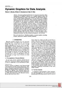
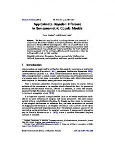
Partitions estimated under the finite mixture/BIC strategy exhibit fair agreement with that estimated using the stochastic DPM method. However, the number of identified outliers is generally greater, illustrating that the evidence required to detect outliers is somewhat less than the ‘very strong’ requirement imposed by the DPM strategy. The MAP estimation results illustrate a multi-way balance among utility, computational expense, accuracy, and stochasticity. For instance, the Gibbs method and other MCMC methods yield good posterior estimates and have high utility in applications beyond MAP estimation. However, the utility of MCMC methods comes with greater computational expense. The agglomerative and stochastic methods have less utility, but offer less computational burden. The agglomerative method is deterministic, but does not guarantee accurate MAP estimates. The SUGS method generates partition estimates quickly, but is not competitive with respect to log posterior mass. However, the SUGS++ results indicate that the SUGS strategy may be modified to accommodate MAP estimation with little or no additional computational burden. The fair agreement in Rand index between the SUGS and ‘Stochastic’ partitions may partially explain why the SUGS method yields reasonable predictions in nonparametric applications, despite having smaller posterior mass. Figure 1 illustrates the MAP data partition for 297 genes regulated in the G1 phase. The MAP data partition for the G1 phase consisted of 12 outlier clusters accounting for 19 outlier observations. In order to illustrate inference using the outlier detection criterion presented in Section 2, consider the set of data partitions that might be formed by merging the outlier cluster in the upper righthand corner of Figure 1 with one of the remaining clusters. Specifying α = 1/150 ensures that the Bayes factor for the MAP partition versus any such partition takes a value greater than 150. Hence, there is ‘very strong’ evidence for the decision to identify this cluster as an outlier. Figure 2 summarizes the five MAP estimates by collapsing clusters according to the outlier cluster size rule (i.e. clusters having n(k) ≤ 3 are labeled outliers). Because distinct clusters have dissimilar mean expression profiles, collapsed observations in the ‘non-outlier’ and ‘outlier’ panels of Figure 2 may appear inhomogeneous. This reflects the possibility that multiple outlier and non-outlier clusters are present in each panel, and does not indicate poor sensitivity or specificity to detect outliers. The distinction between outlier and non-outlier clusters is made on the basis of cluster size. That is, small clusters are considered outliers, for some notion of smallness in a particular data problem (e.g. nk smaller than 1% of n). More importantly, when α = 1/150, there is ‘very strong’ evidence that gene expression profiles assigned to dif-


681

20 60 100

Normalized Expression

2 1 0 −1 −2

2 1 0 −1 −2

2 1 0 −1 −2

20 60 100

n=1

n=2

n=2

n=1

n=1

n=3

n=4

n=2

n=2

n=1

n=5

n=1

n=2

n=4

n=1

n=11

n=4

n=4

n=6

n=10

n=107

n=81

n=20

n=6

n=16

20 60 100

20 60 100

2 1 0 −1 −2

2 1 0 −1 −2

20 60 100

Time (min) Figure 1: Gene expression profiles from the ‘alpha’ synchronized experiment for 297 genes regulated in the G1 phase of the cell cycle (Spellman et al. 1998). Each panel represents a cluster of genes identified by the MAP estimated data partition. Light gray lines give the expression profiles for each gene. Black lines give the profile posterior mean function for each cluster. The values of n are the number of expression profiles presented in each panel.

ferent clusters in the MAP estimate indeed arose from distinct processes. This property holds regardless of what size cluster is considered small.

682


20

original

outliern=18

outliern=20 G2

G2

non−outlier n=99

outliern=19

2 1 0 −1 −2

G1

non−outlier n=278 G1

original n=297

2 1 0 −1 −2

M

M

M

non−outlier n=175

original n=119

60

outliern=21 MG1

MG1

non−outlier n=92

original n=193

20

n=9

S

S

S MG1

2 1 0 −1 −2

outlier

n=60

original n=113

G2

2 1 0 −1 −2

100

non−outlier

n=69

G1

Normalized Expression

2 1 0 −1 −2

60

100

20

60

100

Time (min) Figure 2: Gene expression profiles from the ‘alpha’ synchronized experiment for 791 ‘cell cycle-regulated’ genes identified by Spellman et al. (1998). Light gray lines give the expression profiles for each gene. The values of n are the number of expression profiles presented in each panel. Panels in the leftmost column represent the original clusters of Spellman et al. The center and rightmost panels are collated from multiple distinct clusters of the estimated data partition according to the outlier cluster size rule (n ≤ 3).


5

683

Conclusion

The outlier detection criterion of Section 2 offers an inference mechanism that evaluates the Bayes factor between an estimated (MAP) outlier partition, and a broad class of partitions formed by merging outlier clusters. However, the criterion makes no comparison with partitions outside this class. In particular, there is no guarantee that partitions formed by a sequence of merge and split operations will satisfy the criterion. The stochastic MAP estimation algorithm of Section 3 avoids the complexity and expense of posterior sampling. As a result, this method has computational efficiency on par with popular non-Bayesian optimization methods. Still, more tailored strategies are welcome. The work of Dahl (2009) is a pioneering example, where the MAP estimate in a restricted class of augmented DPMs may be found in only n(n + 1)/2 posterior evaluations. Adapting methods from the computer science literature, such as branching and bounding (Laursen 1993), and simulated annealing (Kirkpatrick et al. 1983) may also be fruitful. Because parallel computeing is gaining favor over serial computing, there is a growing need for computational strategies that exploit sophisticated parallelization in multicore and cluster computing environments. Wilkinson (2008) identifies concurrency and simplicity as important qualities in the future of statistical computing.

684

6 6.1


Appendix Algorithm Consistency

Suppose {z(t) } is a sequence of estimates for the data partition MAP estimator zMAP . Let qt be the nonzero probability that z(t) takes on the value zMAP . That is, with probability qt , p(z(t) |y) ≥ p(z0 |y) for all z0 . However, the algorithm of Section 3 stipulates that p(z(t) |y) ≥ p(z(t−1) |y). This implies that qt ≥ qt−1 . Let T be the smallest value of t such that z(t) = zMAP . It is shown that limT 0 →∞ p(T < T 0 ) = 1. This probability is expressed

p(T < T 0 )

=

1 − p(T ≥ T 0 )

= 1 − p(T = T 0 ) − p(T > T 0 ) = 1 − qT 0

0 TY −1

0

(1 − qt ) −

t=0

T Y

(1 − qt ).

t=0

Since qt is a nonzero probability and qt ≥ qt−1 for all t, the limit of p(T < T 0 ) as T 0 approaches infinity is one.

6.2

Covariate Transformation

The following R code was used to transform a time covariate x onto the space spanned by a collection of power and sine functions.

transform