VARSAT: Integrating Novel Probabilistic Inference Techniques with ...

VARSAT: Integrating Novel Probabilistic Inference Techniques with DPLL Search Eric I. Hsu and Sheila A. McIlraith Department of Computer Science University of Toronto {eihsu,sheila}@cs.toronto.edu http://www.cs.toronto.edu/∼eihsu/VARSAT

Abstract. Probabilistic inference techniques can be used to estimate variable bias, or the proportion of solutions to a given SAT problem that fix a variable positively or negatively. Methods like Belief Propagation (BP), Survey Propagation (SP), and Expectation Maximization BP (EMBP) have been used to guess solutions directly, but intuitively they should also prove useful as variable- and valueordering heuristics within full backtracking (DPLL) search. Here we report on practical design issues for realizing this intuition in the VARSAT system, which is built upon the full-featured MiniSat solver. A second, algorithmic, contribution is to present four novel inference techniques that combine BP/SP models with local/global consistency constraints via the EMBP framework. Empirically, we can also report exponential speed-up over existing complete methods, for random problems at the critically-constrained phase transition region in problem hardness. For industrial problems, VARSAT is slower that MiniSat, but comparable in the number and types problems it is able to solve. Key words: Probabilistic Inference, Survey Propagation/EMBP, Variable/Value Ordering Heuristics

1

Introduction

A variety of message-passing (a.k.a. “propagation”) algorithms have been used to estimate variable “bias,” or the probability of finding each variable set one way or another if we could somehow sample from the space of solutions to a given SAT instance. In particular, Belief Propagation (BP) has been used to differentiate solutions where a variable is constrained to be positive from those where it is negatively constrained [1]. Survey Propagation (SP) extends this model to represent a third probability representing solutions where the variable is not constrained at all; on hypothetically sampling we might find that it is set positively or negatively, but flipping it would still result in a solution [2]. Either model can be employed within the Expectation Maximization Belief Propagation (EMBP) framework, a convergent alternative that accommodates a choice of consistency constraints for balancing speed and accuracy in estimating bias [3]. While bias estimators produce intuitively useful information about the solutions of SAT instances, they cannot actually solve a problem on their own. To date they have all employed a “decimation” framework of computing a single sequence of estimates,

2

VARSAT: Integrating Novel Probabilistic Inference Techniques with DPLL Search

while setting a block of one or more most strongly-biased variables after each estimate. Taken with this decimation framework, the probabilistic bias estimators are state-of-theart for solving large random problems near the critically-constrained phase transition in problem hardness [4]. However, this construction cannot backtrack or take advantage of modern advances in systematic DPLL search like clause learning; the decimation process either directly reaches a solution by a series of fortuitous variable assignments, or it ends in failure without determining satisfiability or unsatisfiability. Toward the upper reaches of the phase transition threshold, failure occurs about half the time (at α = 4.4 for satisfiable problems). For industrial SAT problems with “real-world” structure, the combination is entirely unusable [5]. Here we report on the integration of six bias estimators as variable- and valueordering heuristics within the full-featured MiniSat backtracking solver [6]. Moving past basic intuitions and creating a practical solver requires a number of possibly intuitive, but still non-obvious design decisions and optimizations, due especially to the high computational expense associated with bias estimation. A second contribution consists of four novel estimation techniques whose stand-alone accuracy has been summarized elsewhere without explanation–here they are presented in full for the first time [5]. In particular, we employ local or global consistency approximations to extend either the BP or the SP model, producing EMBP-L, EMSP-L, EMBP-G, and EMSP-G. Together with basic BP and SP, these rules drive the resulting VARSAT solver, so-named in recognition of the variational methods underlying the estimators [7]. VARSAT retains the superior performance of probabilistic techniques on hard random problems, but represents a first step toward handling industrial problems as well. On the latter, its performance is comparable to regular MiniSat in that they are both able to solve mostly the same problems within a given time limit; the main difference is that VARSAT is slower to solve the same problems. The following two sections provide further background and formal definitions concerning propagation algorithms and their application to SAT. Next, Section 4 presents the six bias estimators alongside intuitive explanations of how they work. Then, Section 5 discusses their integration within backtracking DPLL search, and Section 6 summarizes the main experimental findings. Lastly, Section 7 extracts overall conclusions and discusses future work.

2

Background

Message-passing algorithms have been applied to a growing variety of combinatorial problems [2, 8–10], augmenting their traditional roles in probabilistic inference [11– 13]. The methods all operate by propagating messages between a problem’s variables, causing them to iteratively adjust their own bias estimates from some initial randomized values. The techniques produce “surveys”, representing, informally, the probability that each variable should be set a certain way if we were to assemble a satisfying assignment. Thus a propagation algorithm does not output an outright solution to a SAT problem. Rather, applying a probabilistic method to SAT-solving requires two interrelated design decisions: a means of calculating surveys, and a means of using the surveys to fix the


3

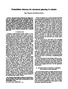
next variable within an arbitrary search framework. A reasonable strategy for the second step is to pick the variable with the most extreme bias, and set it in the direction of that bias, i.e. “succeed-first” search. But by better understanding the characteristics of various survey techniques, we can explore more sophisticated approaches to variable and value ordering. Note also that integrating with a solver will mean computing a new survey each time we fix a single variable; in other words the size of a decimation block will be one. This is a standard practice for addressing correlations between variables [3]; A single survey might report that v1 is usually true within the space of solutions, and that v2 is usually false, even though the two events happen simultaneously with relative infrequency. Instead of attempting to fix multiple variables at once, then, we will fix a single first and simplify the resulting problem. In subsequent surveys the other variables’ biases would thus be conditioned on this first assignment. At a high level, propagation techniques accomplish the bias estimation task by passing messages over a given SAT problem’s “factor graph” representation, as depicted in Figure 1. Nodes representing variables connect to “factor” nodes representing clauses in which they appear. Edges can be distinguished, conceptually, by whether the variables appear as positive or negative literals in the clauses. Thus, for example, we see that factor f1 realizes the disjunction x1 ∨ x2 ∨ ¬x3 . The example problem has nine solutions, as listed in Figure 2. From this table we can calculate exact biases by tallying entries along each column: for instance x1 is set positively in six out of the nine solutions, and negatively in the remaining three. (This calculation glosses the notion of variables being constrained positively or negatively, versus merely appearing as such; this is the distinction between BP and SP.) Conceptually, edges carry clause-to-variable messages in one direction, and variableto clause messages in the other. For all the techniques presented shortly, each variable is first randomly seeded with an initial bias, and informs all of its clauses by passing variable-to-clause messages along the edges. The clauses compile such reports and determine whether they are poorly supported–that is, they calculate the probability that their variables will jointly end up failing to satisfy them. From here they signal each variable as to whether they need their support by passing messages back along the edges, in the opposite direction. The variables weigh such requests, and begin a new iteration by updating and reporting their new biases. Importantly, though, the entire factor graph framework is notional in the sense that it formalizes the derivation of our bias estimators [5], but they will never actually represent such a structure in memory, or organize a series of messages. This is crucial to the efficient implementation of such methods; in the end we will instead use a set of update rules whereby a given variable’s bias is directly updated via a fixed calculation in terms of the biases of adjacent variables (that is, those with which it appears together in some clause.)

3

Definitions

Definition 1 (SAT instance) A (CNF) SAT instance is a set C of m clauses, constraining a set V of n Boolean variables. Each clause c ∈ C is a disjunction of literals built

4

VARSAT: Integrating Novel Probabilistic Inference Techniques with DPLL Search SAT Theory: C1 ∧ . . . ∧ C8 C1 C3 C5 C7

= (x1 = (x1 = (x1 = (x2

∨ x2 ∨ ¬x2 ∨ ¬x3 ∨ x4

∨ ¬x3 ) ∨ ¬x5 ) ∨ x5 ) ∨ x5 )

C2 C4 C6 C8

= (¬x1 = (¬x1 = ( x1 = (¬x3

∨ ¬x2 ∨ x3 ∨ ¬x4 ∨ x4

f7

∨ ¬x4 ) ∨ ¬x4 ) ∨ x5 ) ∨ ¬x5 )

f8 X4

X5

f4

f3 X2

f6

f2

X3 f5

X1 variable appears positively in clause:

variable appears negatively in clause:

f1

Fig. 1. Example 3-SAT Problem: as Factor Graph and as CNF Theory.

from the variables in V . An assignment X ∈ {0, 1}n to the variables satisfies the instance if it makes at least one literal true in each clause. The sets Vc+ and Vc− comprise the variables appearing positively and negatively in a clause c, respectively. The sets Cv+ and Cv− comprise the clauses that contain positive and negative literals for variable v, respectively. Cv = Cv+ ∪ Cv− comprises all clauses that contain v as a whole. Definition 2 (Bias, Survey) For a satisfiable SAT instance F, the bias distribution θv of a variable v represents the fraction of solutions to F wherein v appears positively or negatively. Thus it consists of a positive bias θv+ and a negative bias θv− , where θv+ , θv− ∈ [0, 1] and θv+ + θv− = 1. A vector of bias distributions, one for each variable in a theory, will be called a survey, denoted Θ(F). Less formally, it is useful to describe a variable as “positively biased” with respect to a true or estimated bias distribution. This means that under the given distribution, its positive bias exceeds its negative bias. Similarly the “strength” of a bias distribution indicates how much it favors one value over the other, as defined by the maximum difference between its positive or negative bias and 0.5.

VARSAT: Integrating Novel Probabilistic Inference Techniques with DPLL Search x1 h 0, h 0, h 0, h 1, h 1, h 1, h 1, h 1, h 1,

x2 0, 0, 1, 0, 0, 0, 1, 1, 1,

x3 0, 0, 0, 0, 1, 1, 0, 0, 1,

x4 0, 1, 0, 0, 1, 1, 0, 0, 0,

x5 1 i 1 i 0 i 1 i 0 i 1 i 0 i 1 i 0 i

θ1 (+) = 6/9, θ2 (+) = 4/9, θ3 (+) = 3/9, θ4 (+) = 3/9, θ5 (+) = 5/9,

5

θ1 (−) = 3/9 θ2 (−) = 5/9 θ3 (−) = 6/9 θ4 (−) = 6/9 θ5 (−) = 4/9

Fig. 2. Solutions to Example 3-SAT Problem, and Resulting Biases.

4

Probabilistic Methods for Estimating Bias

In this section we present six distinct propagation methods for measuring variable bias: Belief Propagation (BP), EM Belief Propagation-Local/Global (EMBP-L and EMBPG), Survey Propagation (SP), and EM Survey Propagation-Local/Global (EMSP-L and EMSP-G). These methods represent the space of algorithms defined by choosing between BP and SP and then employing one of them either in original form, or by applying a local- or global-consistency transformation based on the Expectation Maximization framework. The EM-based rules represent a secondary contribution of this work; they have been studied empirically without explanation [14] but have not been presented up to this point. (Complete derivations are available online [5].) On receiving a SAT instance F, any of the propagation methods begins by formulating an initial survey at random. For instance, the positive bias can be randomly generated, and the negative bias can be set to its complement: ∀v, θv+ ∼ U[0, 1]; θv− ← 1 − θv+ . Each algorithm proceeds to successively refine its estimates, over multiple iterations. An iteration consists of a single pass through all variables, where the bias for each variable is updated with respect to the other variables’ biases, according to the characteristic rule for a method. If no variable’s bias has changed between two successive iterations, the process ends with convergence; otherwise an algorithm terminates by timeout or some other parameter. EM-type methods are “convergent”, or guaranteed to converge naturally, while regular BP and SP are not [3].

σ(v, c) ,

θi−

Q i∈Vc+ \{v}

Q j∈Vc− \{v}

θj+

(a) σ(v, c): v is the sole support of c. θv+ 0 ←

+ ωv

+ − ∗ ωv + ωv + ωv

θv− 0 ←

θv+ 0 ←

+ ωv

+ − ωv + ωv

θv− 0 ←

− ωv

+ − ωv + ωv

(b) Bias normalization for BP methods. − ωv

+ − ∗ ωv + ωv + ωv

θv∗ 0 ←

∗ ωv

+ − ∗ ωv + ωv + ωv

(c) Bias normalization for SP methods. Fig. 3. Formula for “sole-support”; normalizing rules for BP and SP families of bias estimators.

6


The six propagation methods are discussed elsewhere in greater theoretical detail than space permits here [3, 2]. But for a practical understanding, they can be viewed as update rules that assign weights (ωv+ and ωv− ) toward a variable’s positive and negative biases–plus a third weight (ωv∗ ) for the “joker bias” (described below) in the case of SP-based methods. The rules will make extensive use of the formula σ(v, c) in Figure 3(a). In doing so they express the probability that variable v is the “sole-support” of clause c in an implicitly sampled configuration of all the variables: every other variable that appears in the clause is set unsatisfyingly. From a generative statistical perspective, the probability of this event is the product of the negative biases of all other variables that appear in the clause as positive literals, and the positive biases of all variables that are supposed to be negative. The six sets of update rules produce intermediate “weight” values for each variable, by consulting the current biases of its surrounding variables. In the case of BP-based methods, each variable has two weights: one toward the positive, and one toward the negative; introducing the SP model will add a third weight toward the unconstrained state. Such weights are then normalized into proper probabilities as depicted in Figures 3(b) and 3(c), depending on whether we are using the BP or SP model. This probability constitutes a new estimated bias distribution for each variable, completing a single iteration of the algorithm. The update rules are presented below in Figures 4 and 5.

ωv+ =

Q

ωv+ = |Cv | −

(1 − σ(v, c))

− c∈Cv

ωv− =

Q

P

σ(v, c)

− c∈Cv

ωv− = |Cv | −

(1 − σ(v, c))

+ c∈Cv

P

σ(v, c)

+ c∈Cv

(a) Regular BP update rule. " ωv+ = |Cv− |

(b) EMBP-L update rule. # Q

(1 − σ(v, c)) + |Cv+ |

− c∈Cv

" ωv−

=

|Cv+ |

# Q

(1 − σ(v, c)) + |Cv− |

+ c∈Cv

(c) EMBP-G update rule. Fig. 4. Update rules for the Belief Propagation (BP) family of bias estimators.

BP can be viewed at first as generating the probability that v should be positive according to the odds that one of its positive clauses is completely dependent on v for support. That is, v appears as a positive literal in some c ∈ Cv+ for which every other positive literal i turns out negative (with probability θi− ), and for which every negative literal ¬j turns out positive (with probability θj+ ). This combination of unsatisfying events would be represented by the expression σ(v, c). However, a defining characteristic of BP is its assumption that every v is the sole support of at least one clause. (Further,


7

v cannot be the only hope of support both a positive and a negative clause simultaneously, since we are sampling from the space of satisfying assignments.) Thus, we should view Figure 4(a) as weighing the probability that no negative clause needs v (implying that v is positive by assumption), versus the probability that no positive clause needs v for support. EMBP-L is the first of a set of update rules derived using the EM method for maximum-likelihood parameter estimation. This statistical technique features guaranteed convergence, but requires a bit of invention to be used as a bias estimator for constraint satisfaction problems [13, 9]. Resulting rules like EMBP-L are variations on BP that calculate a milder, arithmetic average by using summation, in contrast to the harsher geometric average realized by products. This is one reflection of an EM-based method’s convergence versus the non-convergence of regular BP and SP. All propagation methods can be viewed as energy minimization techniques whose successive updates form paths to local optima in the landscape of survey likelihood [3]. By taking smaller, arithmetic steps, EMBP-L (and EMBP-G) is guaranteed to proceed from its initial estimate to the nearest optimum; BP and SP take larger, geometric steps, and can therefore overshoot optima. This explains why BP and SP can explore a larger area of the space of surveys, even when initialized from the same point as EMBP-L, but it also leads to their non-convergence. Empirically, EMBP-L and EMBP-G usually converge in three or four iterations for the examined SAT instances, whereas BP and SP typically require at least ten or so, if they converge at all. Intuitively, the equation in Figure 4(b) (additively) reduces the weight on a variable’s positive bias according to the chances that it is needed by negative clauses, and vice-versa. Such reductions are taken from a smoothing constant representing the number of clauses a variable appears in overall; highly connected variables have less extreme biases than those with fewer constraints. EMBP-G is also based on smoother, arithmetic averages, but employs a broader view than EMBP-L. While the latter is based on “local” inference, resembling generalized arc-consistency, the derivation of EMBP-G uses global consistency across all variables. In the final result, this is partly reflected by the way that Figure 5(c) weights a variable’s positive bias by going through each negative clause (in multiplying by |Cv− |) and uniformly adding the chance that all negative clauses are satisfied without v. In contrast, when EMBP-L iterates through the negative clauses, it considers their satisfaction on an individual basis, without regard to how the clauses’ means of satisfaction might interact with one another. So local consistency is more sensitive to individual clauses in that it will subtract a different value for each clause from the total weight, instead of using the same value uniformly. At the same time, the uniform value that global consistency does apply for each constraint reflects the satisfaction of all clauses at once. SP can be seen as a more sophisticated version of BP, specialized for SAT. To eliminate the assumption that every variable is the sole support of some clause, it introduces the possibility that a variable is not constrained at all in a given satisfying assignment. Thus, it uses the three-weight normalization equations in Figure 3(c) to calculate a three-part bias distribution for each variable: θv+ , θv− , and θv∗ , where ‘*’ indicates the unconstrained (a.k.a “joker”) state. Thus, in examining the weight on the positive bias

8

VARSAT: Integrating Novel Probabilistic Inference Techniques with DPLL Search " ωv+

=

Q

(1 − σ(v, c)) · ρ 1 −

− c∈Cv

# Q

Q

(1 − σ(v, c)) · ρ 1 −

# Q

(1 − σ(v, c))

ωv− = |Cv | −

ωv∗

Q

=

σ(v, c)

P

σ(v, c)

+ c∈Cv

− c∈Cv

+ c∈Cv

P − c∈Cv

" ωv− =

ωv+ = |Cv | −

(1 − σ(v, c))

+ c∈Cv

ωv∗ = |Cv | −

(1 − σ(v, c))

P

σ(v, c)

c∈Cv

c∈Cv

(b) EMSP-L update rule.

(a) Regular SP update rule. " ωv+

=

|Cv− |

Q

(1 − σ(v, c)) +

|Cv+ |

# Q

1−

− c∈Cv

" ωv−

=

|Cv+ |

Q

(1 − σ(v, c))

+ c∈Cv

(1 − σ(v, c)) +

|Cv− |

# Q

1−

(1 − σ(v, c))

− c∈Cv

+ c∈Cv

ωv∗ = |Cv |

Q

(1 − σ(v, c))

c∈Cv

(c) EMSP-G update rule. Fig. 5. Update rules for the Survey Propagation (SP) family of bias estimators.

in Figure 5(a), it is no longer sufficient to represent the probability that no negative clause needs v. Rather, we explicitly factor in the condition that some positive clause needs v, by complementing the probability that no positive clause needs it. This acknowledges the possibility that no negative clause needs v, but no positive clause needs it either. As seen in the equation for ωv∗ , such mass goes toward the joker state. (The parameter ρ = 0.95 is an optional smoothing constant explained in [15].) For the purposes of estimating bias and finding backbones, any probability mass for θv∗ is evenly distributed between θv+ and θv− when the final survey is compiled. This reflects how the event of finding a solution with v labeled as unconstrained indicates that there exists one otherwise identical solution with v set to true, and another with it set to false. So while the “joker” state plays a role between iterations in setting a variable’s bias, the final result omits it for the purposes of bias estimation. (One point of future interest is to examine the prevalence of lower “joker” bias in backdoor variables [16].) EMSP-L and EMSP-G are analogous to their BP counterparts, extended to weight the third ’*’ state where a variable may be unconstrained. So similarly, they can be understood as convergent versions of SP that take a locally or globally consistent view of finding a solution, respectively.


5

9

Practical Design Considerations

In this section we discuss the most salient design considerations for integrating the rules of the previous section within MiniSat, a backtracking DPLL solver that integrates clause learning, restarts, and pre-processing with a built-in ordering heuristic based on VSIDS [6]. In short, the efficient operation of VARSAT hinges upon the interaction of five principle design decisions: a branching strategy for ordering variables and values, a threshold for deactivating the entire bias estimation apparatus, the decimation block size for fixing variables on completing a survey, a policy for using learned clauses in surveys, and finally, the choice of bias estimation technique. Other than the choice of branching strategy, all of these decisions seek a profitable sacrifice in accuracy in return for spending less time on computing surveys. Here it is important to note that in searching for a satisfying solution, robustness is more important than pure accuracy. Even if our bias estimator instructs us to set a variable positively when its true bias is 90% negative, there still exists some set of solutions in the resulting subproblem. Thus our system would always proceed directly to a solution without even backtracking, so long as we never set a variable to a polarity for which it has a true bias of zero. 5.1

Branching Strategy

We tested several branching strategies for using surveys as variable- and value-ordering heuristics. In addition to the “conflict-avoiding” strategy of setting the most strongly biased variable to its stronger value, we also tried to “fail-first” or streamline a problem via the “conflict-seeking” strategy of setting the strongest variable to its weaker value [17]. Additional approaches involved different ways of blending the two: for instance, one strategy might involve triggering propagations and building up a strong database of learned clauses by seeking conflicts, and then trying to find a solution within this greatly restricted search space by switching to conflict avoidance. A second motivator for seeking conflicts is unsatisfiable problems. While surveys are not well-defined for such problems, seeking conflicts can lead to shorter proofs of unsatisfiability and thus faster run-times; since we must account for the entire breadth of the search tree, we should order variables so that conflicts occur on the shallowest subtrees possible. For mixtures of satisfiable and unsatisfiable problems like those comprising the test cases for recent SAT-Solving contests, it turns out that the single best strategy is the (presumably) most intuitive one of avoiding conflicts. 5.2

Deactivation Threshold

A second consideration when integrating with a backtracking solver is that any of the six bias estimators can be governed by a “threshold” parameter expressed in terms of the most strongly biased variable in a survey. For instance, if this parameter is set to 0.6, then we only persist in using surveys so long as their most strongly biased variables have a gap of size 0.6 between their positive and negative bias. As soon as we receive a survey where the strongest bias for a variable does not exceed this gap, then we deactivate the

10


bias estimation process and revert to using MiniSat’s default variable and value ordering heuristic until the solver triggers a restart. (Note that setting this parameter to 0.0 is the same as directing the solver to never deactivate the bias estimator.) The underlying motivation is that problems should contain a few important variables that are more constrained than the rest, and that the rest of the variables should be easy to set once these few have been assigned correctly. The aim is to detect and fix the first type of variable via strong bias estimates, and then solve the resulting subproblem using DPLL search alone with a default ordering heuristic. For various theoretical reasons, the divide between a small number of constrained variables and a large number of less important ones is thought to be of special relevance within the phase-transition region in hardness for random problems [18]. For industrial and crafted problems, the hope is that a similar distinction exists; but here the exact ratio eludes formal analysis. Most generally, surveys are highly valuable but also very expensive; they can take the majority of a solver’s total runtime depending on how this parameter and others are set. So it is critical to stop computing surveys after the most important decisions have been made. For typical SAT contest problems, we have found .9 to be a good value in combination with the other settings decided in this section. This will typically result in the execution of about one survey per thousand variables before deactivation, for large problems with tens of thousands of variables and up1 (Each time the solver performs a restart in solving a given problem, the bias estimation module is re-instated if it was previously deactivated.) 5.3

Decimation Block Size

Another way to mitigate the high cost of computing surveys is to use a large decimation block size, meaning that we can set a number of variables at once each time we complete a survey. The problem is then simplified via unit propagation and we compute a new survey on the resulting sub-problem. Under preliminary investigation we have found that it is still better to use a block size of 1, though this issue is not fully resolved due to the many combinations of settings for the other parameters discussed so far. As mentioned previously, the motivation for a small decimation size is to account for correlations between variable biases. When setting a block of multiple variables, we are approximating a joint probability over their mutual configuration by the product of their individual marginal probabilities. If we instead set a single variable and compute a new survey, the resulting values are conditioned upon our previous decision. At this point it seems that the extra accuracy provided by this property is worth the greater computational cost. 5.4

Integrating Learned Clauses

Integrating learned clauses into surveys represents another balance between accuracy and runtime efficiency. On the one hand, learned clauses are all implied by a theory, 1

For the smaller problems considered in Figure 6, surveys typically wound up running over approximately a tenth of the total variables in a problem.


11

and their influence is already implicitly captured by the original clauses of a problem. On the other, they may provide especially useful information about the specific area of the search space that a solver is currently exploring. There is an extra cost in runtime because update rules must now iterate through additional clauses when estimating biases; at an implementational level there is also the overhead of managing memory for registering learned clauses to be used in surveys, and for unregistering them when they are periodically purged. The tradeoff is accomplished by a parameter that states the maximum size that a learned clause can have if it is to be used in surveys. (Shorter clauses are more valuable in the sense that they contain more information, and they are also faster to process since they appear in the update rules of fewer variables.) In practice we have found it best to integrate all learned 4-clauses and below into survey computations. For the SATcontest problems considered, though, very few such clauses are ever learned, and the improvement over not using any learned clauses at all is small. 5.5

Bias Estimation Technique

Finally, the choice of bias estimator represents a tradeoff between runtime and various types of accuracy. This decision has the most interaction with the way the other design issues are resolved. For instance, suppose we are decimating one variable at a time and are seeking solutions by branching on the one with strongest estimated bias. Then it does us no good if our chosen estimator has excellent accuracy on the majority of the variables if it often happens that the one variable with strongest estimated bias is guessed incorrectly. For random problems, stronger global constraints and the richer SP model make EMSP-G the best bias estimator, despite the greater cost of computing such constraints and performing three updates per variable instead of two. For industrial problems from recent SAT contests, the global constraints are still valuable but the SP model no longer seems to be worthwhile–here EMBP-G is the method of choice.

6

Empirical Performance

Here we briefly summarize the empirical performance of the completed VARSAT system. More in-depth studies of the individual bias estimators and parameter settings are detailed online [5], while performance on specific data sets will be available when the 2009 SAT contest is completed. Figure 6 compares VARSAT’s heuristic strategy with the default strategy of MiniSat 2.0, on hard random problems of increasing size. Here EMSP-G was used as the bias estimator, with deactivation threshold 0.6, to perform conflict-avoiding search with decimation block size of one and no learned clauses consulted in forming surveys. For each problem size marked in the graph, the two solvers were run on 1000 satisfiable instances that were randomly generated with a clause-to-variable ratio of 4.11– such problems approach the hard region of the satisfiability phase transition. The average runtime on such problems is plotted in log-scale. The last two data points for

12

VARSAT: Integrating Novel Probabilistic Inference Techniques with DPLL Search 10000 +11% timeout

Average Runtime in Seconds / Timeout = 10,800 sec.

+3% timeout 1000

100

10

1

0.1

0.01 ’EMSPG’ ’default’ ’default-lb’ 0.001 50

100

150

200 250 300 350 400 Number of Variables in Problem (n)

Fig. 6. Comparison on Random Problems, n = 50 − 500, α ≡

450

m n

500

= 4.11.

default MiniSat represent lower bounds; on a percentage of the runs MiniSat timed out by failing to solve an instance within 10,800 seconds (three hours.) However, the real strength of MiniSat and other DPLL-based solvers is on industrial problems. While the results of this year’s contest remain to be seen, it is possible to perform a comparison using last year’s data sets. Here the best configuration of VARSAT was to use EMBP-G with a deactivation threshold of 0.9, and the other parameters remaining the same. On running the two solvers on a collection of 125 past problems with a timeout of 15 minutes, they were both able to solve 65 of them, and both failed to solve 46. Of the former, MiniSat was generally faster though both were within the time limit. Additionally, there were 4 problems that only VARSAT could solve, compared to 10 for MiniSat. Other comparisons suggest that the performance of VARSAT relative MiniSat improves given a longer timeout–on the larger problems, bias estimation takes up more than 99% of runtime, and just initializing the appropriate structures can take minutes under the current implementation.

7

Conclusions and Future Work

The main finding of this work has been that probabilistic message-passing techniques can be successfully integrated within a backtracking search framework, in order to achieve completeness and also in order to handle industrial problems. This is contingent on a number of design decisions that primarily trade accuracy for time. A second


13

contribution is four novel bias estimators, two of which (EMBP-G and EMSP-G) have proved to be the most useful within the resulting VARSAT solver. Integrating messagepassing with DPLL combines the best properties of random-walk based methods (good performance on random problems) with backtracking methods (completeness), but in a very simple sense. In terms of raw performance, VARSAT is comparable but still generally slower than MiniSat on non-random problems. However, the overall framework is new and not close to fully explored. The parameters discussed in Section 5 produce a complex of combinations and interactions that should be resolved more systematically according to the type of problem being solved. Statistical analysis provides one automated means for doing so [19, 20]. Unsatisfiable problems are such a type of especial future interest; while the scheme presented here works reasonably well on satisfiable and unsatisfiable problem instances alike, the actual semantics of bias over the latter type of instance eludes easy definition. At any rate it appears likely that a specialized set of parameter settings will improve future efforts to apply VARSAT to unsatisfiable problems. Another task is to speed up the bias estimation process by better optimizing its code at an implementational level, possibly to include porting it to alternative hardware [21]. Algorithmically, an additional possibility is to use only a portion of a variable’s clauses in estimating its bias. There are interesting abstract similarities with other problem-solving methodologies for constraint satisfaction. Bias measures the probability of a variable setting given satisfaction, while many local search methods maximize the probability of satisfaction given a certain variable setting [22]. Thus, the two targets are directly proportional via Bayes’ Rule and techniques for one can be applied to the other. Another line of similar research calculates exact solution counts for individual constraints as a means of ordering variables and values [23]. Fundamentally, such an approach represents an exact and localized version of the approximate and interlinked techniques studied here. Finally, another means to making incomplete search complete is to define a gradient function for local search and register local minima by adding successive constraints until the resulting problem is convex [24]. The probabilistic (marginal computation) methods presented here are not strictly related to local search, but they are very similar to gradient-based (MAP-computation) methods that follow the same framework [7]. Future applications of bias estimation include query answering and model counting. In the case of model counting, one detail omitted from discussion is that the normalization value ωv+ + ωv− in Figure 3(b) (in fact, the log-partition function of a specific Markov Random Field) is proportional to the number of solutions for a given problem.

References 1. Dechter, R., Kask, K., Mateescu, R.: Iterative join-graph propagation. In: Proc. of 18th International Conference on Uncertainty in Artificial Intelligence (UAI ’02), Edmonton, Canada. (2002) 128–136 2. Braunstein, A., Mezard, M., Zecchina, R.: Survey propagation: An algorithm for satisfiability. Random Structures and Algorithms 27 (2005) 201–226

14


3. Hsu, E., McIlraith, S.: Characterizing propagation methods for Boolean satisfiability. In: Proc. of 9th International Conference on Theory and Applications of Satisfiability Testing (SAT ’06), Seattle, WA. (2006) 4. Achlioptas, D., Ricci-Tersenghi, F.: Random formulas have frozen variables. To appear, SIAM Journal of Computing 5. Hsu, E.I.: VARSAT SAT-Solver homepage. http://www.cs.toronto.edu/ ∼eihsu/VARSAT/ (2008) 6. E´en, N., S¨orensson, N.: An extensible SAT-solver. In: Proc. of 6th International Conference on Theory and Applications of Satisfiability Testing (SAT ’03), Portofino, Italy. (2003) 7. Jordan, M., Ghahramani, Z., Jaakkola, T., Saul, L.: An introduction to variational methods for graphical models. In Jordan, M., ed.: Learning in Graphical Models. MIT Press (1998) 8. Kask, K., Dechter, R., Gogate, V.: Counting-based look-ahead schemes for constraint satisfaction. In: Proc. of 10th International Conference on Constraint Processing (CP ’04), Toronto, Canada. (2004) 9. Hsu, E., Kitching, M., Bacchus, F., McIlraith, S.: Using EM to find likely assignments for solving CSP’s. In: Proc. of 22nd Conference on Artificial Intelligence (AAAI ’07), Vancouver, Canada. (2007) 10. Kroc, L., Sabharwal, A., Selman, B.: Survey propagation revisited. In: Proc. of 23rd International Conference on Uncertainty in Artificial Intelligence (UAI ’07), Vancouver, Canada. (2007) 11. Pearl, J.: Probabilistic Reasoning in Intelligent Systems. Morgan Kaufmann, San Mateo (1988) 12. Kschischang, F.R., Frey, B.J., Loeliger, H.A.: Factor graphs and the sum-product algorithm. IEEE Transactions on Information Theory 47(2) (2001) 13. Dempster, A., Laird, N., Rubin, D.: Maximum likelihood from incomplete data via the EM algorithm. Journal of the Royal Statistical Society 39(1) (1977) 1–39 14. Hsu, E., Muise, C., Beck, J.C., McIlraith, S.: Probabilistically estimating backbones and variable bias: Experimental overview. In: Proc. of 14th International Conference on Constraint Processing (CP ’08), Sydney, Australia. (2008) 15. Maneva, E., Mossel, E., Wainwright, M.: A new look at survey propagation and its generalizations. Journal of the ACM 54(4) (2007) 2–41 16. Williams, R., Gomes, C., Selman, B.: Backdoors to typical case complexity. In: Proc. of 18th International Joint Conference on Artificial Intelligence (IJCAI ’03), Acapulco, Mexico. (2003) 17. Beck, J.C., Prosser, P., Wallace, R.J.: Trying again to fail-first. Recent Advances in Constraints, Lecture Notes in Artificial Intelligence 3419 (2005) 18. Braunstein, A., Zecchina, R.: Survey propagation as local equilibrium equations. Journal of Statistical Mechanics: Theory and Experiments PO6007 (2004) 19. Wallace, R.J.: Factor analytic studies of CSP heuristics. 3709 (2005) 712–726 20. Xu, L., Hutter, F., Hoos, H.H., Leyton-Brown, K.: SATzilla: portfolio-based algorithm selection for SAT. Journal of Artificial Intelligence Research 32 (June 2008) 565–606 21. Manolios, P., Zhang, Y.: Implementing survey propagation on graphics processing units. In: Proc. of 9th International Conference on Theory and Applications of Satisfiability Testing (SAT ’06), Seattle, WA. (2006) 22. Zhang, W.: Configuration landscape analysis and backbone guided local search. Part I: Satisfiability and maximum satisfiability. Artificial Intelligence 158(1) (2004) 1–26 23. Zanarini, A., Pesant, G.: Solution counting algorithms for constraint-centered search heuristics. In: Proc. of 13th International Conference on Constraint Processing (CP ’07), Providence, RI. (2007) 24. Fang, H., Ruml, W.: Complete local search for propositional satisfiability. In: Proc. of 19th National Conference on Artificial Intelligence (AAAI ’04), San Jose, CA. (2004)