Bayesian inferential framework for diagnosis of non-stationary systems Vadim N. Smelyanskiya , Dmitry G. Luchinskya , Andrea Duggentob and Peter V. E. McClintockb a NASA
Ames Research Center, MS 269-3, Moffett Field, CA 94035-1000, U.S. Department, Lancaster University, LA1 4YB, Lancaster, U.K.
b Physics
ABSTRACT A Bayesian framework for parameter inference in non-stationary, nonlinear, stochastic, dynamical systems is introduced. It is applied to decode time variation of control parameters from time-series data modelling physiological signals. In this context a system of FitzHugh-Nagumo (FHN) oscillators is considered, for which synthetically generated signals are mixed via a measurement matrix. For each oscillator only one of the dynamical variables is assumed to be measured, while another variable remains hidden (unobservable). The control parameter for each FHN oscillator is varying in time. It is shown that the proposed approach allows one: (i) to reconstruct both unmeasured (hidden) variables of the FHN oscillators and the model parameters, (ii) to detect stepwise changes of control parameters for each oscillator, and (iii) to follow a continuous evolution of the control parameters in the quasi-adiabatic limit. Keywords: Nonlinear time-series analysis, Bayesian inference, varying parameters, FitzHugh-Nagumo, measurement matrix.
1. INTRODUCTION The ubiquity of noisy nonlinear systems in nature has led to the use of stochastic nonlinear dynamical models for observed phenomena across many scientific disciplines, including the modelling of biological nonstationary signals. Important “hidden” features of a model such as coupling coefficients between the dynamical degrees of freedom can be very difficult to extract due to the presence of intrinsic dynamical noise and the intricate interplay between noise and nonlinearity. The problem becomes even more challenging if we want to detect and characterize the nonstationarity of the system following the evolution of system’s parameters. Fast (almost real-time) detection of parameters’ evolution is essential in the identification, diagnostic, and prognostic of the time evolution of complex dynamical systems. This is especially true when dealing with biological signals. In our earlier work1 an efficient technique of Bayesian inference of nonlinear noise-driven dynamical models that guarantees optimum compensation of dynamical noise-induced errors for continuous systems and avoids extensive numerical optimization was introduced. In the present paper we extend earlier results and introduce a Bayesian framework for inferring parameters of continuous non-stationary systems, and in particular for the long standing problem of reconstruction of parameters for neuronal systems. Neuronal signals are a good example, for which the Bayesian inference is especially advantageous: often the system’s dynamical details are known only approximately. There is a strong influence from internal noise but, most of all, the coefficients and coupling terms are in general not constant, and so a fast and “elastic in adaptation” technique is needed to detect changes of the system. In this context a system of FitzHugh-Nagumo (FHN) oscillators is considered, for which synthetically generated signals are mixed via a measurement matrix. For each oscillator only one of the dynamical variables is assumed to be measured, while another variable remains hidden (unobservable). The control parameter for each FHN oscillator is varying in time. The goal is to decode a control parameter for each signal. Note that Further author information: (Send correspondence to A.D.) A.D.: E-mail:
[email protected], Telephone: +44 (0) 1524 593206, Address: Department of Physics, Lancaster University, Lancaster LA1 4YB, U.K.
the system of FitzHugh-Nagumo oscillators is one of the most useful models2–4 in explaining a lot of different biological dynamics. It can present spontaneous oscillatory firing patterns5 and it can be used to characterize electrical signal propagation in nerve fibres6 and in cardiac tissue.7–9 The paper is organized as follows. First, we describe how the Bayesian algorithm is applied to a single oscillator, and then we discuss a multi-dimensional system, where every signal coming from a FitzHugh-Nagumo oscillator is linearly mixed with the other ones through a specific mixing measurement matrix. We then provide practical demonstration of how model parameters and noise coefficients can be inferred in this situation, and consider the advantages and limitation of this present technique.
2. BACKGROUND ON BAYESIAN INFERENCE Let us suppose we have to analyse a signal coming from an L-dimensional system of the form x˙ = f (x|c) + ξ(t) !ξ(t)" = 0,
ˆ δ(t − t! ) !ξ(t) ξ T (t! )" = D
(1)
where c is a vector of unknown parameters and ξ(t) is a white Gaussian additive dynamical noise characterized by ˆ The task is to decode the optimal set of parameters M = {c, D}, ˆ given a set of measurement diffusion matrix D. X. A priori knowledge of Mis summarized in the so-called prior probability density function (PDF) ppr (M). Then the time-series X is acquired from the experimental set up, and the new gained information is used to compute the a posteriori PDF of the model parameters, namely ppost (M|X ). The relationship between the two distribution ppr (M) and ppost (M|X ) is given by the Bayes’ theorem: ppost (M|X ) = !
"(X |M) ppr (M) . "(X |M) ppr (M) dM
(2)
The PDF "(X |M) (also called likelihood of X ) is the conditional probability of the occurrence of measurements X when the set of parameters M is given. The procedure can be applied iteratively for a sequence of data blocks {X1 , X2 , . . . }: the posterior for one block is the the prior for the next block: ppr (Mi+1 ) = ppost (Mi |Xi ) The densities ppost for each Mi are a sequence of functions that become sharper and sharper functions that peak at the solution of the inference problem. One of the main goals of dynamical inference is to find the correct analytical expression for the likelihood and to introduce an efficient algorithm for optimization of the posterior distribution with respect to the model parameters. Both problems are very non trivial in the context of nonlinear dynamical stochastic systems. In the earlier research the correct analytical form for "(X |M) could not be found and optimization was mainly relying on extensive numerical methods. In a recent work1 we have introduced (and verified in application to the dynamical inference of cardio-vascular system? ) analytical solution for a wide class of non-linear stochastic systems which does not require extensive numerical calculations and provides an optimal compensation for the noise-induced errors. One of the keys of the novel approach is to write the expression for the likelihood in the form of a path integral over the random trajectories of the system: " x(tf ) "(X |M) = FM [x(t)] Dx(t), (3) x(ti )
A very important step in calculation of this integral is to write the correct form of the Jacobian of transformation from stochastic to dynamical variables. It is the analytical factor related to this Jacobian of transformation that guarantees the optimal compensation of the noise-induced errors by providing a leading order contribution to the analytical expression for the posterior PDF. Another key is to introduce a convenient parameterizations of the vector field. We now briefly summarize the results of these calculations.
2.1 Parameterization of the vector field and likelihood construction We assume that the data block of measurement X ≡ {x(tk ), k = 1, . . . , K} comes from an uniform time grid: xk ≡ x(tk ) tk = t0 + k h, tK − t0 h= K
(4) (5)
k = 1, . . . , K.
(6)
With this discretization, the system in (1) might be approximated as: x˙ k+1 = xk + h f (x∗k |c) + ξk ˆ δs q !ξk " = 0, !ξs ξq T " = D
(7)
where use of the following definition was made: x∗k =
xk+1 − xk 2
!t and the vector ξk = tkk+1 ξ(s)ds. on the uniform time lattice the discretized version of the logarithm of the likelihood takes the form: % % K−1 $ $ K h # ∂f (x∗k |c) T ˆ −1 ∗ ∗ ˆ ˙ ˙ (8) log "(X |M) = − ln det D − tr + (xk − f (xk |c)) D (xk − f (xk |c)) + I. 2 2 ∂x k=0
Here we have introduced the “velocity” x˙ k
x˙ k ≡ h−1 (xk+1 − xk ). and I is a constant factor which depends on neither M nor X . It should be noted that, in general, the likelihood in eq.(8) is such that the integral " "(X |M) p(M) dM
which appears in eq.(2) does not have a closed analytic solution. To overcome this problem authors of? proposed the following parameterizations of the vector field: ˆ f (x|c) ≡ U(x) c u1 (x) ˆ U(x) ≡
..
. u1 (x)
uN (x) ...
..
.
uN (x)
where {u1 (x), . . . , uN (x)} is a set of suitable base functions. With this parameterization we assume that the function f (x), which is nonlinear in respect of x, might be expressed as a weighted sum of nonlinear base functions. Parameters c are the weights of this sum. Note that f (xk |c) might be highly non linear in x, and we are only assuming linearity in respect of parameters. In this way the likelihood function became a multivariate normal distribution in respect of c. Thus, for a ˆ taking the initial prior ppr (c) to be a multivariate normal distribution centered in some prior mean cpr given D, ˆ pr , the posterior ppost (c) is also Gaussian. So the algorithm for finding both c and and with prior covariance Σ ˆ might be a two step optimization process which performs iteratively the following two operations: (i) given D ˆ (ii) given D, ˆ compute the best choice of c. The details of the algorithm have c, compute the best choice of D; ˆ if been given elsewhere? but a few comment will be made. The quantity to be maximized in respect of c, and D the negative logarithm of the posterior is ˆ = SX (c, D)
1 ˆ ˆ + 1 cT Ξ(D)c. ˆ ρ(D) − cT w(D) 2 2
(9)
Figure 1. Synthetic data for one uncoupled FHN system. (a) x(t) and q(t), (b) limit cycles (solid line) and isoclines: −x1 (x1 − θ1 )(x1 − 1) − q1 + η1 = 0 (dashed line); βx1 − γ1 q1 = 0 (bold dashed line). Parameters are: γ1 = 0.0051051, β = 0.0051, α1 = 0.2, η1 = 0.112, and d1 = 1 × 10⁻⁵ .
where the following definitions has been used ˆ ≡h ρ(D)
K−1 #
ˆ −1 x˙ k + K ln(det D), ˆ x˙ Tk D
k=0
ˆ ≡Σ ˆ −1 w(D) pr cpr + h ˆ ≡Σ ˆ −1 Ξ(D) pr + h
K−1 # k=0
K−1 #
,
(10)
L ∗ # 1 ∂u (x ) l k ˆ T (x∗k ) D ˆ −1 x˙k − , U 2 ∂xl
(11)
l=1
ˆ T (x∗k ) D ˆ −1 U(x ˆ ∗k ) . U
(12)
k=0
ˆ and the next step parameter vector is c! = Ξc, where at each steps Ξ−1 is the new covariance matrix given D, ˆ ˆ is given D; while, given c, the maximum of the negative logarithm of posterior in respect of D K−1 /T . / #. ˆ = h ˆ kc ˆ kc . D x˙ k − U x˙ k − U K
(13)
k=0
3. THEORY OF DECOUPLING OF A NUMBER OF FITZHUGH-NAGUMO SYSTEMS MIXED BY MEASUREMENT MATRIX In this section we will take into consideration the signal coming from a FitzHugh-Nagumo model. This is a widely used model for the neuron dynamic2–5 and, in particular, for nerve fibres6 and heart tissues.7–9 It consist of two coupled first order differential equation described by the variable x and q. x is the membrane potential, w is a recovery variable, slower than x.5 A set of multiple neurons can be written as: x˙ j = −xj (xj − αj ) (xj − 1) − qj + ηj + ξj , q˙j = −β qj + γj xj , !ξj (t) ξi (t! )" = di j δ(t − t! ),
(14)
i, j = 1 : L.
j labels all the L neurons, and at the membrane potential a white Gaussian noise is present. Parameters ηj , αj , γj are possibly different for each neuron. In particular ηj has a special importance since it models the input current at the membrane and it acts as a control parameter for the firing frequency, related to the information transfer in physiological systems. It is particularly important in the view of the physiological applications to decode this parameter. Note that, in general, parameter β also has to be inferred. However, in what follows we will assume for the sake of simplicity that it is a known constant for each neuron.
Figure 2. Model of measurements assumes that x1 (t) and x2 (t) are mixed with known matrix X as in (23). (a) x1 (t) (black solid line) and x2 (t) (grey dotted line), (b) y1 (t) (black solid line) and y2 (t) (grey dotted line). Parameter as in Table 4.1.
Note also that, in practice, the signal from different neurons are mixed by a measurement matrix X, so it would be useful to have a technique to decode these parameter from a corresponding readout variable related to the membrane potentials via the following expression: yi = Xij xj
(15)
Where yi represents the output of our signal, i.e. see Fig. (2). With this approach we have to find the basis functions u(y1 , . . . , yL ) such that the systems # y˙ i = ai j uj (y1 , . . . , yL ) j
represents the dynamics of measured variables corresponding to the underlying dynamics of actual variables described by eq.(14) and measurement model given by (3). First q has to be reconstructed, since it is not read directly. We solve equation eq.(14), that is: " t qj (t) = γ dτ exp(−β (t − τ )) xj (τ ) + exp(−βt)qj (0) 0
Here qj (0) is a set of initial coordinates that needs to be inferred along with the rest of parameters. We plug this equation into eq.(14) and obtain: " t x˙ j (t) = −xj (xj − αj ) (xj − 1) + ηj + dj − γ exp(−β (t − τ ))xj (τ )dτ + exp(−βt)qj (0) . (16) 0
!t
The function 0 exp(−β (t − τ ))xj (τ )dτ is defined over the time grid {t0 , t1 , . . . , tN }. After some algebraic manipulations, using trapezoidal rule for the evaluation of the integral, it can be shows that "
0
tk
exp(−β (t − τ ))xj (τ )dτ = h
N #
n=0
xj (tn ) exp (β(tn − tN )) −
h (xj (t0 ) exp(β(t0 − tN )) + xj (tN )) . 2
Substituting eq.(16) into eq.(15) we obtain finally the required system of equations in the form: y˙ j =
N #
Aj i yi +
i=1
−
N #
Bj k1 k2 yk1 yk2 +
k1,k2=1
"
t
t0
dτ
N #
i,k=1
exp[−β (t −
N #
Cj k1 k2 k3 yk1 yk2 yk3 +
k1,k2,k3=1
τ )] Γji k yk (τ )
−
N # i=1
exp[−β t] q˜j + η˜j +
N # i=1
(17) Dj i ξi (t).
Here, use was made of the following definitions: Aj k =
N # i=1
1 0 Xj i αi X −1 i k ,
Bj k1 k2 =
N #
i,k1 ,k2 =1
0 1 0 1 Xj i (1 + αi ) X −1 i k X −1 i k 1
N #
Cj k1 k2 k3 =
i,k1 ,k2 ,k3 =1
Γji k
2
(18)
1 0 1 0 1 0 Xj i X −1 i k1 X −1 i k2 X −1 i k3 ,
0 1 = Xj i γi X −1 i k .
The modified noise intensities Dj for an auxiliary system (3) are expressed in terms of dj , and the modified initial condition for q˜i are expressed in terms of qj as follows: Dj =
N #
q˜j =
X j i di
i=1
N #
Xj i qi (0).
(19)
i=1
The parameters η˜j that appear in eq.(17) are related to the original model parameters ηj , as follows: η˜j =
N #
Xj i ηi . .
(20)
i=1
From eq.(17), we can see that if the system’s dimension L increases, and if we cannot make any assumption on the form of the coupling, the increase in the number of parameters is proportional to L3 . In aprticular, when L = 2, the following base functions have to be used to infer matrix elements of A, B, C, Γ, D, η˜: u1 ≡ 1
u2 ≡ y 1
u3 ≡ y2
u4 ≡ y12
u5 ≡ y22
u6 ≡ y1 y2
u7 ≡ y13
u11 ≡ h
y1 (l) exp (β(tl − tk )) −
h (y1 (0) exp(β(t0 − tk )) + y1 (k)) , 2
y2 (l) exp (β(tl − tk )) −
h (y2 (0) exp(β(t0 − tk )) + y2 (k)) 2
u12 ≡ h
k # l=0
k # l=0
u8 ≡ y12 y2
u9 ≡ y1 y22
u10 ≡ y23 (21)
u13 ≡ − exp(β(t0 − tk )) . Thus the total number of parameters is 26 and the vector c as a function of the parameters’ matrix elements takes the form c = [˜ η1 , η˜2 , −A11 , −A21 , −A12 , −A22 , . . . B111 , B211 , (B112 + B121 ), . . . (B212 + B221 ), B122 , B222 , −C1111 , −C2111 , . . . .
−(C1112 + C1121 + C1211 ), −(C2112 + C2121 + C2211 ), . . . −(C1122 + C1221 + C1212 ), −(C2122 + C2221 + C2212 ), . . . −C1222 , −C2222 , γ1 , γ2 , q˜1 , q˜2 ] .
(22)
4. INFERENCE OF THE CONTROL PARAMETERS FOR TWO COUPLED FHN SYSTEMS In this section the inference algorithm described above will be tested using synthetically generated signal for the system of two FHN oscillators. First, we will describe how the signal is generated and how the stream of data
is passed on to the inferring machinery; then tests of convergence will be carried out in the case of a stationary dynamic; finally a demonstration and consideration of how the technique performs in the case of a non-stationary dynamics will be presented.
4.1 Synthetic data and preliminary test To test our inferential algorithm we generate 2 signals from a 2-dimensional FHN system as in eq.(14), keeping all parameters fixed. To generate the stream of data, the stochastic differential equation has been integrated accordingly to the Heun scheme.10 In Fig. (2) (a) a sample of data generated with coefficent as in Table (4.1) is shown. The signals yi obtained multiplying the mixing matrix with the signals xi is the imput for the algorithm. α1 = α2 = β1 = β2 = d11 = d22 =
0.2 0.2 0.0051 0.0051 0.004 0.004
η = η = γ1 = γ2 = d12 = d21 =
0.15 0.15 0.0051051 0.0051051 0.001 0.001
Table 1. Values of coefficients for the generated stationary signal
The measurement matrix has been taken in the following form: $ % 1 2 X= 2 1
(23)
In this way we generate contiguously multiple blocks of points. Values of the control parameters η1 and η2 change step-wise at random from block to block and remain constant within each block. Other parameters of the system remain constant all the time. The inference is performed through the following steps: 1. Use a non-informative prior for parameters with an infinitely large variance. block 2. Compute the first block p1st (M). post
3. Reset the prior to an infinitely large multivariate gaussian distribution for each block of data. In Figs.(3)(a) and (b) inferred values of the parameter ηi are compared with their actual values for five time steps. The sampling rate was approximately 50 kHz, i.e. we use 20000 points to infer values of the model parameters on one time step. As it is shown in the figure, the time interval between steps is approximately 5-10 periods of firing of action potential. The measured trajectories y1 (t) and y2 (t) are shown in the Fig. (3) (b) and (e). In the Fig. (3) (c) and (f) we compare the reconstructed dynamic variable qi for each oscillator. In order to obtain the unmeasured coordinate qi (t) the second line of eq.(14) has been integrated numerically using inferred coefficients, and using the boundary condition qi (0) that can be derived from eq.(19): qi (0) =
N #
Xi−1 ˜j j q
.
(24)
j=1
4.2 Test of convergence It is also advisable to check how the convergence depends on the total time of measurements of the time-series data. To this end we generate synthetic time-series data keeping all coefficients constant and express he total measurement time as the number of blocks. A ensemble of different sample signals (number of runs) is generated for each value of the total measurement time and inference procedure is carried out independently for each run. Statistical properties from the ensemble of inferred parameters computed in this way provide an example of the convergence of coefficients ci as shown in Fig. (4). The number of runs to obtain the averaged convergence was 3000 for each size of the block of data. It can be seen from the figure that the time of convergence is larger
for the coefficients corresponding to higher powers of the dynamical variables in the equations. Convergence of the diffusion coefficients is shown in Fig. (5). As it can be seen that the inferred parameters for diffusion ˆ are on average overestimated compared to the real ones. This behavior is rather simply explained: matrix D ˆ is given by eq.(13). Nevertheless it holds for real coefficients c. the maximum of the likelihood in respect of D In our case the vector c is not exact, but it represents the maximum of the likelihood in respect of vector c, thus ˆ reflects the propagation of the uncertainly it is a statistical quantity. Thus, the slight bias in the estimation of D ˆ and c in a loop until convergence is in the inferred c. To avoid this bias one has to repeat calculations of D reached as will be explained in details elsewhere. The coefficients presented in Figs. (4) and (5) are the weight factors for the base functions of eq.(21). To reconstruct the original coefficients, and to check the quality of our estimation, we recover coefficients (14) and the elements of the diffusion matrix di using eqs.(20) that are reduced in our case to the following expressions: A = X −1 AX, ˜ Γ = X 1 ΓX,
(25) (26)
D=X
−1
˜ T )−1 , D(X
(27)
η=X
−1
η˜.
(28)
Here A is a diagonal matrix with diagonal elements equal to α1 and α2 , Γ is a diagonal matrix with diagonal elements equal to γ1 and γ2 . Since in our test α1 = α2 , γ1 = γ2 and η1 = η2 we present the results of recovering of the original coefficients only for the first equation. The results of the inference of the original equations obtained from the inference of the mixed equations with the help of relations (28) are shown in Fig. (6). For the block of data containing 8000 points, results of the inference are summarized in Table 2.
4.3 Parameters η If we devote our attention only to the inference of parameters η1 and η2 , namely if prior knowledge of all the other parameters is given, clearly we need much less information (sample data) to achieve good estimations of ηi . As has been done formerly, η1 and η2 change step-wise at random and remain constant between steps. However, the time interval between steps is now 20 times smaller and is less then one period of firing of an action potential.
Figure 3. Inference of the model parameters of two uncoupled FHN systems mixed by the measurement matrix with step-wise changes of η1 and η2 . (a) Actual values of η1 are shown by solid lines in comparison with inferred values shown by dotted lines. (b) Measured mixed values of coordinates y1 (t) (solid line). (c) Mixed value of the generated coordinate q1 (t) is shown in comparison with its inferred value integrated from q˜i . Figures (d), (e), and (f) show the corresponding result for the second system. The values of other parameters were α1 = α2 = 0.2, β = 0.0051051, γ1 = γ2 = 0.0051.
Figure 4. Convergence of some of the model parameters ci as a function of the length of the block of data. The sampling rate is approximately 50 kHz. First point corresponds to the 1000 data points in one block. For each next point the number of data points was increased by 1000. Vertical lines shows standard deviation of the inferred values of the model coefficients. The horizontal dashed lines shows actual values of the model parameters. The values of other parameters were α1 = α2 = 0.2, β = 0.0051051, γ1 = γ2 = 0.0051.
Figure 5. Convergence of the diffusion coefficients as a function of the length of the block of data. Parameters are the same as in Fig. (4).
Other parameters of the system remain constant all the time. At each step we infer only parameters η1 and η2 of the model assuming their initial values to be zero and their initial dispersion to be infinity. In Fig. (7) inferred values of the parameter ηi are compared with their actual values for five time steps. The sampling rate was approximately 50 kHz, i.e. we use 1000 points to infer values of the model parameters in each time step. The measured trajectories y1 (t) and y2 (t) are shown in the Fig. (7) (b) and (e). The values of the real and inferred coordinates qi (t) are compared in Fig. (7) (c) and (f). The results obtained so far show a remarkably close correspondence between the real and inferred values, but one can argue that this correspondence is due to the fact that real parameters ηi change stepwise but remain constant during each block of inference. Therefore, in the following we will investigate the possibility of inference in case of continuous smoothly-varying parameters η1 and η2 that have both periodic and random components. Although the algorithm is the same, the data set now consists of a series of blocks 10000 points long each; i.e. we have a few periods of firing per one block of inference. We also assume that all other parameters of the system are known. The results of inference are shown in the Fig. (8). The results are very similar to those shown in the Fig. (7) except that we now infer the average value of ηi per block. This result suggests that we can obtain a better approximation of the actual values of η by shifting the initial time of each block and assuming that the inferred value of ηi corresponds to the time at the middle point of the block. It is clear that thanks to this “block by block” approach the quality of inference for smoothly-varying parameters seems to fulfill the researcher’s expectation; thus, to complete the scenario of the inference of multiple
Figure 6. Convergence of the original coefficients (a) η1 , (b) α1 , (c) γ1 , and (d) d1 as functions of the time if inference was conducted with a sampling rate of 55 kHz. Parameters are the same as in Fig. (4).
η1 0.112 0.1245 0.0097
α1 0.2 0.2161 0.0202
γ1 0.0051 0.0055 0.0003
d1 0.001 0.0010 0.0003
Table 2. Values of the original coefficients inferred using 8000 points measured with sampling rate 55 kHz obtained from mixed measurements with the help of eqs. (28). The actual values (top row) are compared with the inferred values (middle row), standard deviations are given in the bottom row.
parameters, we present the performances of the algorithm in case when all parameters need to be inferred. Hence, in the next and last part no assumptions are made, nor prior knowledge of others parameters taken as given, and η1 and η2 are varying with periodic and random components. The results for a block of data containing 8000 points results of inference are summarized in Table 3. At each step of the algorithm we use the c1 0.1106 0.2084 c7 1.2000 1.2174 c18 0.6667 1.5529
c2 0.0607 0.2074 c8 0.8000 0.9871 c19 -0.2222 -0.3399
c3 -0.2000 -0.2130 c9 -1.6000 -1.5712 c20 -0.5556 -0.7994
c4 0 -0.0062 c10 -1.6000 -2.0007 c21 0.0051 0.0049
c5 0 0.0130 c11 0.8000 -1.0123 c22 0.7500 0.7255
D11 0.0009 0.0010 D12 0.0006 0.0006 D22 0.0009 0.0010
Table 3. Values of some model coefficients inferred at the first step. The actual values (top row) are compared with the inferred values (bottom row).
coefficients of the model inferred at the previous step to infer ηi parameters. We use a sampling rate of 55 kHz and 15000 points per block of inference. The results are shown in Fig. (9). They are very similar to those shown of Fig. (8) even though the values of the model coefficients are now known only approximately, thus confirming on the efficacy of the technique for parameter-tracking purposes.
5. CONCLUSION In this paper we have presented a new application of the Bayesian dynamical inference technique. To the previously proposed method1 additional features have been added, namely we have taken into account the variability of parameters of the model that has to be inferred. Here (a) driving parameters that are varying in time have been infered in a dynamical system of coupled FHN oscillators with additive noise, and (b) the general framework of application the Bayesian algorithm to a multiple FHN system has been presented.
Figure 7. Inference of η1 and η2 for two uncoupled FHN systems mixed by the measurement matrix. (a) The actual values of η1 , are shown by solid lines, are almost indistinguishable from the inferred values, shown by dotted lines. (b) Measured mixed values of coordinates y1 (t) (solid line). (c) Values of the coordinate q1 (t) are shown in comparison with its inferred value. Figures (d), (e), and (f) show the same results for the second system. The values of other parameters where α1 = α2 = 0.2, β = 0.0051051, γ1 = γ2 = 0.0051.
Figure 8. Inference of smoothly-varying η1 and η2 that have both periodic and random components for two uncoupled FHN systems. (a) Actual values of η1 are shown by black solid lines in comparison with inferred values shown by gray dotted lines. (b) Measured mixed values of coordinates y1 (t) (solid line). (c) Values of the coordinate q1 (t) (solid line) is almost indistinguishable from the inferred value (gray dotted line). Figures (d), (e), and (f) show the same results for the second system. The values of other parameters where α1 = α2 = 0.2, β = 0.0051051, γ1 = γ2 = 0.0051.
As readout variables we considered a vector formed from a linear combination of the system dynamical variables mixed through a measurement matrix. The multiple FHN system here is therefore taken in general form. This allows us to demonstrate that it is possible to recover the real system parameters and the diffusion coefficients. As a result we have shown that new algorithm is advantiously fast in detecting dynamic controlling parameters, and it appears to be a desirable and flexible instrument in analysing the data, because it maximises the use of
Figure 9. Inference of smoothly-varying η1 and η2 that have both periodic and random components for two uncoupled FHN systems using model coefficients inferred at the first step. (a) Actual values of η1 are shown by black solid lines in comparison with inferred values shown by gray dotted lines. (b) Measured mixed values of coordinates y1 (t) (solid line). (c) Values of the coordinate q1 (t) are almost indistinguishable from the inferred value (gray dotted line). Figures (d), (e), and (f) show the same results for the second system. The values of other parameters where α1 = α2 = 0.2, β = 0.0051051, γ1 = γ2 = 0.0051.
the available information. Indeed, we have demonstrated it by performing tests where stepwise changes of the dynamics were read under several hypotheses about the factual external knowledge. Due to these properties our inferrence algorithm is also able to follow continuous changes of a system’s parameters. In fact it makes it possible to refresh the inferred system’s state instantaneously (providing opportunity for the model to reflect parameter changes on a continuous time basis).
REFERENCES 1. V. N. Smelyanskiy, D. G. Luchinsky, D. A. Timucin, and A. Bandrivskyy, “Reconstruction of stochastic nonlinear dynamical models from trajectory measurements,” Physical Review E (Statistical, Nonlinear, and Soft Matter Physics) 72(2), p. 026202, 2005. 2. R. FitzHugh, “Impulses and physiological states in theoretical models of nerve membrane,” Biophysical Journal 1(6), pp. 445–466, 1961. 3. J. Nagumo, S. Animoto, and S. Yoshizawa, “An active pulse transmission line simulating nerve axon,” Proc. Inst. Radio Engineers 50, pp. 2061–2070, 1962. 4. A. T. Winfree, The Geometry of Biological Time, Springer-Verlag, New York, 1980. 5. E. Izhikevich, Dynamical Systems in Neuroscience: The Geometry of Excitability and Bursting., MIT Press, 2005. preprint. 6. J. Keener and J. Sneyd, Mathematical Physiology, Springer-Verlag, New York, 1998. 7. E. N. Best, “Null space in the hodgkin-huxley equations - a critical test,” Biophysical Journal 27(1), pp. 87– 104, 1979. 8. J. Rogers and A. McCulloch, “A collocation-galerkin finite element model of cardiac action potential propagation,” IEEE Trans. Biomed. Eng. 41, pp. 743–757, 1994. 9. R. R. Aliev and A. V. Panfilov, “Modeling of heart excitation patterns caused by a local inhomogeneity,” Journal of Theoretical Biology 181(1), pp. 33–40, 1996. 10. R. Mannella, “Integration of stochastic differential equations on a computer,” International Journal of Modern Physics C 13(9), pp. 1177–1195, 2002.