BAYESIAN METHOD FOR SEGMENTATION OF SAR IMAGES IN ROUGH TERRAIN Marco Caparrini1 , Klaus Seidel1 , and Mihai Datcu2 1
2
Computer Vision Laboratory, ETH Z¨ urich Gloriastr. 35, CH-8092 Z¨ urich Phone: +41 1 632 4261, Fax: +41 1 632 1251, Email: {mcaparri,seidel}@vision.ee.ethz.ch German Aerospace Center (DLR), Remote Sensing Technology Institute (IMF) D-82234 Weßling Phone: +49 8153 28 1388, Fax: +49 8153 28 1448, Email:
[email protected]
ABSTRACT Radiometric correction is the essential prerequisite to obtain precise and valuable segmentation of remote sensing images, especially when dealing with mountainous regions where the terrain is more likely to be rough. Important applications such as snow cover segmentation have usually to be performed on images of very rough mountainous terrain where this preprocessing step turns out to be especially demanding. The knowledge of the topography of the imaged area through a digital elevation model (DEM) and of the backscatter function for the different terrain cover types are the basis for radiometric correction. Considering SAR images, the huge amount of processing for geographic and geometric calibration and registration that is needed prior to analysis is well established. Nonetheless, even assuming that these calibration and registration steps can been carried out with high precision algorithms, they are still prone to inaccuracies due to the quality of the terrain geometrical description. In the following is presented a model-based method that, exploiting the information contained both in the DEM and in the image, provides improved estimates, in a Bayesian framework, of the terrain itself and of the radiometric characteristics of the land cover.
INTRODUCTION Scene understanding of remote sensing images requires a certain amount of preprocessing in order to remove or alleviate the effects of all those factors disturbing the imaging process. Radiometric distortions depend essentially on the peculiar way in which a sensor acquires the image (sensor-related factors), on the terrain topography, the illumination and the view angle (terrain-related factors), and on the terrain cover type. The strong influence of topography in remote sensing images is well known and in particular the problem of terraininduced effects and their correction has been addressed in several publications, (1, 2, 3, 4, 5, 6, 7, 8) among others. In particular, in (2) a removal of the topographic information from images is obtained using high resolution digital elevation models and an average backscatter curve. In (8) the information provided by low resolution DEMs and high resolution images are used together to solve the problem of surface topography estimation. In (5) the sine of the local incidence angle is assumed as projection factor for radiometric slope correction. In (4) the cosine of the tilt angle in the azimuth direction is also taken into account, assuming a “separable” projection factor. In (6) a new equation for the projection between ground and image coordinates is derived so that the resulting projection factor is more precise and the two previously cited methods are demonstrated to be just further approximation. In (7) the calibration is mainly based on the evaluation of a real local illuminated area through the knowledge of high resolution DEMs. Once the topographic component of an image has been removed, the thematic information must be extracted in order to achieve the goal of the scene understanding. As a matter of fact it is clear that the two problems are not independently solvable: either the knowledge of the backscatter function is (more or less) arbitrarily assumed, or the topography of the scene is considered to be known up to a sufficient degree. In this paper, a Bayesian model-based maximum a posteriori (MAP) estimation approach to simultaneously perform these corrections and to estimate the backscatter parameters is suggested. The overall idea (Figure 1) is to define a procedure for a high precision MAP segmentation of the image and a concurrent interpolation of a DEM, given a parametric model of the backscatter function and a SAR image of the same area with an higher resolution, exploiting all the information contained in the image itself.
Figure 2: In order to solve the estimation problem (i.e. an inversion problem) the highest possible number of physical phenomena involved in the image formation process should be taken into account.
Figure 1: Diagram of the estimation procedure for a MAP segmentation of the image, exploiting, besides the SAR image and the DEM, parametric models for the terrain, the sensor, and the backscatter function.
IMAGE FORMATION MODEL As a means to define the problem within a Bayesian framework, it is necessary to statistically describe all the phenomena involved. In general, the image formation process (Figure 2) can be seen as a three-stage procedure (9) (10). The first step is the illumination of the scene that has to be imaged with some kind of radiation. The scene will reflect a certain amount of radiation according to its geometrical and physical characteristics: shapes, shadows, roughness, density, humidity among others. This radiation, that represents the second step of the image formation process, that we call ”cross-section”, brings some knowledge about the scene. It represents the future image at its best, in the sense that the information content about the scene enclosed in the final image will be less than or equal to the one incorporated in this so-called cross-section. The third step is the generation of the image by the sensor. The incident field on the sensor is different from the one at the cross-section because of the modifications induced by the propagation through the atmosphere (absorption, diffusion and scattering phenomena). Additionally, the way the sensor itself acquires the signal introduces distortion and noise. In conclusion, the final image results in a 2-dimensional, distorted and noisy representation of the imaged scene.The above process is summarised by the following three elements: the scene, the cross-section , and the image. For our purposes, we must describe this process in a stochastic way, using appropriate probability density functions (pdfs). Assuming that vector δ contains all the parameters describing the geometrical properties of the scene, the probability density function p∆ (δ), together with an appropriate backscatter model, is regarded as the scene model (i.e. the first step in the image formation process as described before). Being x the intensity process of the cross-section (whose dependence on the backscatter model is enclosed in the parameter vector θ), the pdf pX (x|δ, θ) represents the stochastic counterpart of the cross-section (the second step). The propagation through the atmosphere and the sensor image acquisition are modelled by an operator H plus stochastic noise: y = H(x) + n. Finally, the image is represented by the probability density function pY (y|x,n). With this notation, the proposed scene understanding problem, i.e. the estimation of θ (segmentation) and of δ (DEM interpolation) from the observed data y, can be seen as a maximum a posteriori estimation on the posterior probability density function p∆,Θ (δ, θ|y, n). All these probability density functions must be precisely defined.
TERRAIN MODEL As clearly results from the previous section, a model for the imaged terrain must be chosen to determine the p∆ (δ). The need for good DEMs in order to perform the radiometric correction on remote sensing images often comes up against the lack of elevation data with high enough spatial resolution. In this regard, some significant values are listed in Table 1. The interpolation of DEMs is therefore a usual task to be carried out. All interpolation methods, implicitly or explicitly, postulate a model for the terrain. The choice of a model is nothing but a constraint on some characteristic of the imaged land: constraint on the surface structure (bilinear, cubic interpolators), or on the
2
Table 1: Resolutions comparison
vehicle Landsat 7 SPOT 2,3 IKONOS-1 IRS ERS SRTM RADARSAT E-SAR PHARUS CRL/NASDA
sensor or mode
res. [m]
ETM/PAN XS/PAN MSS/PAN PAN/LISS AMI-SAR X-SAR standard/fine (airborne) (airborne) C-band (airborne) X/L-band
30/15 20/10 4/1 1.8/23 30 25 25/8 12 4 1.5/3
DEM source US Geological survey Swiss Fed. Office Topog. Istit. Geog. Militare Italiano SRTM DEM
name “gtopo 30” “1 arc-sec” “RIMINI” “DHM25”
res. [m] 1000 30 250 25 20 30
surface spectrum bandwidth (“sinc” interpolators), or on both the surface structure and its spectrum shape (fractal, Gauss Markov Random Fields interpolators). Moreover, a model is, by definition, an approximation of reality, i.e. some characteristics of the true represented phenomena are lost. For example, real terrains are not stationary. If this feature is considered to be essential for the modelling, then the bilinear, cubic and sinc interpolators are to be excluded. In the following, the fractal model for the terrain will be assumed. The Earth surface, due to its self-similarity properties has been often described by the non-stationary stochastic model of fractional Brownian motion (fBm). This implies the normal distribution of the height increments in different positions of the surface (11) (12). The fractal behaviour of a surface has to be proved using a self-similarity condition. Usually, this condition is verified just in a certain range of scales, i.e. it is possible to find different ranges of scales in which the self-similarity condition holds locally . In each scale range, the stochastic model has consequently a different parameter value, that is the fractal dimension of the surface is different (13). Actually, the measurability of the fractal behaviour of a terrain and its fractal dimension depends strongly on the way the DEM has been derived and represented. Once the fractality of the scene under observation (or part of it) has been proved, at least in the range of scales of interest, its fractal dimension is estimated. Various algorithms (14) have been proposed for measuring this quantity: estimation in the frequency domain, intensity-based estimation, differential box-counting, wavelets (15), morphological approach. The self-similarity condition relates the fractal dimension to the variance of the Gaussian distribution describing the height increments between DEM points at different scales. Using the estimated fractal dimension and according to the self-similarity condition, it is then possible to evaluate the variance of the Gaussian distribution of the increments at a given (finer) scale.
BACKSCATTER MODEL The backscatter model, i.e. the function describing the reflection process, defines the pdf pX (x|δ, θ) and is strongly dependent on the kind of sensor we are dealing with and on the land cover type. For SARs, many models have been developed. A list of some of the empirical backscatter models proposed in literature can be found in (16) and (3). According to (17), most of them can be derived from the general one: x = a · cos(η)c + b, where x is the pixel grey level, η is the local incidence angle and a, b and c are the backscatter model parameters, that is the elements of our vector θ. It is evident that from this general model, the Lambertian model, proved to be appropriate at least for some class of terrain cover type (18), can be derived.
SENSOR IMAGING MODE Another phenomenon to analyse is the way in which the EM wave colliding with the sensor is transformed into an image so that the probability density function of the image given the cross section pY (y|x) can also be defined. Let us consider the case of SARs. Without taking into consideration the terrain cover type but focusing on the orography of the surface, the backscatter coefficient map measured by the SAR system is just a 2 dimensional projection, in the slant range plane, of a three dimensional landscape. This projection is affected by a huge number of system dependent factors and point dependent factors: Earth curvature and rotation, antenna pattern, platform attitude, local incidence angle among others. For these reasons, the mapping of the backscatter coefficient map from the slant range plane back to the ground plane (i.e. the process of geocoding), especially
3
for mountainous areas is not trivial (foreshortening) and under certain conditions it is almost impossible (layover and shadowed areas) (19). Keeping all these factors in mind, under not too restrictive conditions and approximations, the end-to-end SAR system can be modelled as a linear filter plus noise (16). This means that the radar backscatter coefficient map σ o (r, t), convolved with the impulse response of the SAR system |s(r, t)|, provides the map of the expectation of the image intensity value E{i(r, t)}. The assumptions for this scheme to hold are: the start - stop approximation (20); the rectilinear geometry; the scene coherence; the ideal wave propagation in the atmosphere. Another predominant characteristic of SAR imaging system, as a coherent imaging system, is the presence of speckle. When considering an uncorrelated speckle noise, the probability density function of the image given the cross-section is (21) L
y 2
L pY (y|x) = 2( xy )2L−1 xΓ(L) exp−L( x )
where x and y are respectively the square root of the cross-section intensities and the square root of the observed intensities.
DEM & SAR IMAGE INTERDEPENDENCIES In this section the strong connection between the DEM and the SAR image is further elucidated. Consider the two-dimensional situation described in Figure 3(a). Given two points of a height profile, the goal is to interpolate
(a) In this exemplification, an overestimation of the height of the interpolated point leads, on the right (respectively left) slope, to an overestimation (respectively underestimation) of the local incidence angle. The vice-versa holds for an underestimation of the interpolated point height.
(b) Different value of the height of the interpolated point cause different predicted values for the corresponding image gray level (representation consistent with the right slope in the figure on the left).
Figure 3: Interdependencies between DEM interpolation and backscattering.
between them, i.e. to fix a new point whose height value is in some way related to its neighbours’. In Figure 3(a), three possible choices if the height of the interpolated point are marked. It is evident that the three alternatives lead to three different local-incident-angle values. This is shown, for the right side slope, in Figure 3(b). For the three-dimensional case, suppose to have a DEM with a resolution twice coarser than the respective image. The value of the interpolation of a fifth point given four points of the coarse DEM (Figure 4) defines the four local incidence angles, one for each of the sub-facet in the finer DEM. In this Figure, s is the vector identifying the sensor position. If δ is the displacement of the interpolated point w.r.t. the linear interpolation, to obtain the pX (x|δ, θ), the distribution of the cosine of the incidence angle η, cos(η), is necessary. Indicating with the subscript i the magnitudes relative to each of the four local incidence angles (Figure 4), the relation between cos(ηi ) and δ is δ+Ai cos(ηi ) = Ki √δ2 +B , δ+C i
i
4
i = {0, x, xy, y}
nxy
s
Qxy n0
Qy
s
δ
Q0
Qx
Figure 5: Different kinds of interpolators have been compared, on a simulated image, to the interpolation provided by the the estimation procedure proposed. The experiment has been run with different surface roughness, “c” backscatter parameter values and speckle noise distributions.
Figure 4: Geometry for the 3D case DEM interpolation with four local incidence angles.
where Ki are function of s, Ai are function of d (coarse grid resolution), zx , zxy and zy , Bi are function of s, d, zx , zxy and zy , and Ci are function of zx , zxy and zy . To calculate the new pdf, we need the inverse functions (dropping for clearness the subscript i) δ = f (cos(η)). Then another change of variable, from cos(η) to x, is needed to calculate the p(x|δ, θ). The result of this calculations is not easy to handle and approximating functions might be used in order to reach meaningful closed-form equations.
MAP ESTIMATOR As stated in a previous section, the probability density function that we have to maximise to find the MAP estimator of δ and θ is p∆,Θ (δ, θ|y). Using Bayes’ relation: Z p∆,Θ (δ, θ|y) ∝ pY (y|δ, θ) p∆,Θ (δ, θ) = p∆,Θ (δ, θ) pY (y|x, δ, θ) pX (x|δ, θ) dx X
Since the magnitudes related to the backscatter function and those related to the terrain model are independent and since the probability density function of the image given the cross-section is independent of the terrain model and of the backscatter function, the above equation becomes: Z p∆ (δ, θ|y) ∝ p∆ (δ) pΘ (θ) pY (y|x) pX (x|δ, θ) dx X
In p∆ (δ) is contained the prior information about the geometry of the surface. This pdf is clearly determined by the choice of the terrain model. The choice of the backscatter model influences the pΘ (θ) which brings the information about the backscatter-model parameters. The pY (y|x), as already mentioned, is the likelihood of the image given the cross-section 1 , i.e. it is determined by the sensor model. The last factor, pX (x|θ) represents the relation between the cross-section and the backscatter-model parameters.
FEASIBILITY EXPERIMENTAL EVALUATION The following experiment (Figure 5) has been carried out to provide a first evidence of the feasibility of the presented approach. The starting point for this experiment is a 10-metre resolution DEM of a mountainous area in Davos region, in the Swiss Alps. Assuming a certain backscatter function, a simulated SAR image is generated. The simulation considered only the phenomenology relevant for the actual case study. The DEM has been subsequently decimated and interpolated with different interpolators (bilinear, cubic, cubic spline) and 1 No
additive noise is considered
5
according to our method. To evaluate the results, the mean of the absolute difference between the real DEM and the interpolated ones are then compared.
(a) In this case, the real spatial resolution of the DEM has been used.
(b) Same as (a) but assuming a fictitious resolution of the DEM, thus actually considering a rougher terrain.
Figure 6: Mean absolute errors between the real DEM and the interpolated ones. The estimation procedure has been carried out for different values of the backscatter model parameter “c” and of the equivalent number of looks. The interpolation of the DEM exploiting the intensity information provided by the image, can achieve a better result than standard deterministic procedures, especially for very rough terrains.
This experiment has been repeated using different values for the backscatter-model parameter “c” and for various equivalent number of looks. As expected, and as shown in Figure 6(a), the more the backscatter function is shaped, i.e. the higher the value of c, the better is the estimation. The same trend holds when lowering the speckle noise, i.e. increasing the equivalent numbers of looks. If the same experiment is performed using an unrealistic rougher terrain obtained by decreasing the nominal resolution of the original DEM (thus increasing its average slope), better results are obtained, as reported in Figure 6(b). This fact was predictable since a rougher surface means higher contrast among neighbouring pixels. This implies more information brought by the image to the estimation algorithm. In Figure 7, a short profile extracted from the original DEM is shown together with the cubic interpolation of the subsampled DEM and with the points obtained via MAP estimation. Again, in areas with stronger discontinuities, the MAP estimation achieves its best results.
Figure 7: Interpolated height-profile comparison. Where the terrain presents important discontinuities (for example around values 75-80 on the x-axes), the estimation procedure has enough information to overcome the speckle noise and to provide better results than standard deterministic procedures.
Another proof of this behaviour comes from a tentative experiment executed with an ERS 1/2 images pair, 6
with its corresponding interferometric DEM, both provided by the German Aerospace Center DLR (Deutsches Zentrum f¨ ur Luft- und Raumfahrt) in Oberpfaffenhofen. Although the experimental results are currently under evaluation, in Figure 8 two short profiles are shown. The first one (Figure 8(a)) comes from a very rough area and the estimation procedure is on the average more precise than a cubic interpolation. The second profile (Figure 8(b)) is taken from a smoother region and the estimation procedure almost coincides with the cubic interpolation.
CONCLUSION In this paper an original approach to feature extraction from SAR images of rough terrain has been presented. Working in a model-based Bayesian framework, the various sources of information and misinformation (i.e. different kind of noise) can be handled at once. This leads to a unique algorithm capable of simultaneously estimating backscatter features and of improving knowledge about the imaged terrain.
(a) Rough terrain region.
(b) Smooth terrain region.
Figure 8: Interpolated height-profile comparison. The meaning is the same as for Figure 7. This time the estimation was performed on an ERS 1/2 images pair, with corresponding interferometric DEM.
REFERENCES 1. P.T. Teillet. Image correction for radiometric effects in remote sensing. International Journal of Remote Sensing, 7(12):1637–1751, 1986. 1 2. G. Domik, F. Leberl, and J. Cimino. Dependence of image gray values on topography in SIR-B images. International Journal of Remote Sensing, 9(5):1013–1022, 1988. 1 3. T. Bayer, R. Winter, and G. Schreier. Terrain Influences in SAR Backscatter and Attempts to their Correction. IEEE Transactions on Geoscience and Remote Sensing, 29(3):451–462, May 1991. 1, 3 4. J.J. Van Zyl, B.D. Chapman, P. Dubois, and J. Shi. The effect of topography on SAR calibration. IEEE Transactions on Geoscience and Remote Sensing, 31(5):1036–1043, September 1993. 1 5. F. Holecz, E. Meier, J. Piesbergen, D. N¨ uesch, and J. Moreira. Rigorous derivation of backscattering coefficient. IEEE Geoscience and Remote Sensing Soc. Newslett., 92:6–14, 1994. 1 6. L.M.H. Ulander. Radiometric slope correction of synthetic-aperture radar images. IEEE Transections on Geoscience and Remote Sensing, 34(5):1115–1122, September 1996. 1 7. D. Small, F. Holecz, E. Meier, D. N¨ uesch, and A. Barmettler. Geometric and Radiometirc Calibration of RADARSAT Images. In Geomatics in the Era of RADARSAT, May 1997. Ottawa, Canada. 1 8. R.T. Frankot and R. Chellappa. Estimation of Surface Topogrphy from SAR Imagery Using Shape from Shading Techniques. Artificial Intelligence, 43:271–310, 1990. 1
7
9. M. Datcu and G. Schwarz. The Application of Forward Modeling as a Data Analysis Tool. In C.H. Chen, editor, Information Processing for Remote Sensing, pages 51–65. World Scientific, 1999. 2 10. M. Datcu, K. Seidel, and M. Walessa. Spatial information retrieval from remote sensing images Part A: Information theoretical perspective. IEEE Transactions on Geoscience and Remote Sensing, 36(5):1431– 1445, September 1998. 2 11. B.B. Mandelbrot and J.W. Van Ness. Fractional Brownian Motions, Fractional Noise and Applications. SIAM Review, 10:422–437, October 1968. 3 12. L.M. Kaplan and C.-C.J. Kuo. An Improved Method for 2-D Self-Similar Image Synthesis. Transactions on Image Processing, 5(5):754–761, May 1996. 3
IEEE
13. N. Yokoya and K. Yamamoto. Fractal-Based Analysis and Interpolation of 3D Natural Surface Shapes and Their Application to Terrain Modeling. Computer Vision, Graphics, and Image Processing, 46:284–302, 1989. 3 14. Y. Liu and Y. Li. Image Feature Extraction and Segmentation using Fractal Dimension. In International Conference on Information, Communication and Signal Processing, volume 2, pages 975–979, September 1997. 3 15. L.M. Kaplan and C.-C.J. Kuo. Fast Fractal Feature Extraction for Texture Segmentation using Wavelets. In Neural and stochastic methods in image and signal processing III, volume 2304 of SPIE, pages 144–155. The International Society for Optical Engineering, 1994. 3 16. R. Bamler and B. Sch¨ attler. SAR Data Acquisition and Image Formation. In Gunter Schreier, editor, SAR geocoding : data and systems, pages 53–102, Karlsruhe, 1993. Wichmann. 3, 4 17. P. Taillet et al. Slope-Aspect Effects in Synthetic Aperture Radar Imagery. Canadian Jornal of Remote Sensing, 11(1):39–50, 1985. 3 18. S. Paquerault and H. Maˆitre. A new method for backscatter model estimation and elevation map computation using radarclinometry. In F. Posa, editor, SAR Image Analysis, Modeling, and Techniques, volume 3497 of SPIE Proceedings, pages 230–241, September 1998. 3 19. B. Sch¨ attler. SAR geocoding: data and systems, chapter 4. Addison-Wesley, Karlsruhe, 1993. 4 20. B.C. Barber. Theory of digital imaging from orbital synthetic-aperture radar. International Journal of Remote Sensing, 6(7):1009–1057, 1985. review article. 4 21. J.W. Goodman. Statistical Properties of Laser Speckle Patterns. In J.C. Dainty, editor, Laser Speckle and related Phenomena. Springer, 1975. 4
8