Nonlin. Processes Geophys., 18, 515–528, 2011 www.nonlin-processes-geophys.net/18/515/2011/ doi:10.5194/npg-18-515-2011 © Author(s) 2011. CC Attribution 3.0 License.
Nonlinear Processes in Geophysics
Bayesian neural network modeling of tree-ring temperature variability record from the Western Himalayas R. K. Tiwari1 and S. Maiti2 1 National 2 Indian
Geophysical Research Institute (CSIR), Hyderabad-500007, India Institute of Geomagnetism (DST), Navi-Mumbai-410218, India
Received: 21 December 2010 – Revised: 29 July 2011 – Accepted: 30 July 2011 – Published: 5 August 2011
Abstract. A novel technique based on the Bayesian neural network (BNN) theory is developed and employed to model the temperature variation record from the Western Himalayas. In order to estimate an a posteriori probability function, the BNN is trained with the Hybrid Monte Carlo (HMC)/Markov Chain Monte Carlo (MCMC) simulations algorithm. The efficacy of the new algorithm is tested on the well known chaotic, first order autoregressive (AR) and random models and then applied to model the temperature variation record decoded from the tree-ring widths of the Western Himalayas for the period spanning over 1226–2000 AD. For modeling the actual tree-ring temperature data, optimum network parameters are chosen appropriately and then crossvalidation test is performed to ensure the generalization skill of the network on the new data set. Finally, prediction result based on the BNN model is compared with the conventional artificial neural network (ANN) and the AR linear models results. The comparative results show that the BNN based analysis makes better prediction than the ANN and the AR models. The new BNN modeling approach provides a viable tool for climate studies and could also be exploited for modeling other kinds of environmental data.
1 1.1
Introduction General information on predicting temperature
Tree rings provide information about the past natural climate variation at decade to century time scales. This often uses dendroclimatic reconstruction to extend the length of an instrumental climatologically record (Cook, 1985; Briffa et al., 2001; Cook et al., 2003; Esper et al., 2003). The study of tree-ring temperature variation data is useful for Correspondence to: R. K. Tiwari (rk
[email protected])
understanding the past seasonal temperatures or precipitation/drought changes (Crowley, 2000; Jones and Mann, 2004; Woodhouse, 1999; Helama et al., 2009). The physical implications of these studies are discussed in details by several researchers (Cook, 1985; Briffa et al., 2001; Cook et al., 2003; Esper et al., 2003; Jones and Mann, 2004; Boreux et al., 2009; Helama et al., 2009). However the key problem of understanding the nonlinear climate system and predicting the future and/or characterizing the model on the basis of collected data, assumes immense significance both for science and society. Various techniques of time series analysis have invariably been applied to predict the future behavior of climate by extracting the knowledge from the past. In particular there are basically two approaches that have been applied for climate modeling as well as nonlinear time series analyses (Zhang et al., 1998; Tiwari and Srilakshmi, 2009). The first one is a construction of a dynamical model using a set of non-linear ordinary differential equations which can be solved by applying a well specified initial and boundary condition. The second approach has been mainly focused on to the search of some possibility of empirical regularities in the underlying time series using the modern spectral and the nonlinear forecasting approaches (Zhang et al., 1998; Tiwari and Srilakshmi, 2009). However in case of nonlinear dynamic modeling, the available information is often partial and incomplete. In the time series analysis, evidence for empirical regularities or periodicities is not always possible and can often be masked by a significant amount of noise (Zhang et al., 1998; Mihalakakou et al., 1998; Mongue-Sanz and MedranoMarqu´es, 2002; Tiwari and Srilakshmi, 2009). Furthermore, prediction based on these models and techniques crucially depends on the assumption made about the underlying data trend (Mihalakakou et al., 1998). The existing techniques, therefore, either fail in delivering accurate results in most of the cases or at best give vague results that are hardly ever acceptable (Mihalakakou et al., 1998; Mongue-Sanz and Medrano-Marqu´es, 2002).
Published by Copernicus Publications on behalf of the European Geosciences Union and the American Geophysical Union.
516 Nonlinear relationships between the tree growth and the temperature change have long been recognized by dendochronologists (Fritts, 1969, 1991; Gramlich and Brubaker, 1986). However several earlier studies have shown that the tree growth-climate relationships derived from dendroclimate signal becomes complicated owing to population dynamics (Lindholm et al., 2000; Helama et al., 2009). Thus the decoded temperature variations from the tree rings would most likely pose the complex nonlinear problem. The tree ring growth is further controlled by multiple factors that include the temperature and the precipitations besides having several other influences (Helama et al., 2009). Variations in seasonal precipitation could influence the tree ring growth as well and can be to some extent independent of temperature variations too. Hence long-term trends in the underlying data sets could result in nonstationarity/nonlinearity in the width temperature relationship involving different time scales (Helama et al., 2009). The presence of nonstationarity/non-linearity in the data could thus invalidate linear modeling approaches. During the recent years the techniques based on ANNs have been applied for the analyses of various kinds of nonstationary and nonlinear time series data and have proved quite effectual in extracting the useful information from such records (Zhang et al., 1998; Mihalakakou et al., 1998; Maiti and Tiwari, 2010a). The ANN based techniques have favorably fair advantages over the traditional methods in dealing with nonlinearities and noisy input signals. There are many algorithms that have been proposed for ANN learning. Among them the back-propagation (BP) method (Rumelhart, 1986) is more popular which uses the gradient decent scheme for network optimization. It is slow and often gets trapped in one of the many local minima of complex error surface. Consequently to evade this problem, many improvements have been put forward, such as the inclusion of momentum variable, adaptive learning rate (Poulton, 2001; Maiti et al., 2007), conjugate gradient (Bishop, 1995), scaled conjugate gradient (Bishop, 1995; Maiti and Tiwari, 2010b), Levenberg-Marquaard (Bishop, 1995; Poulton, 2001). Recently several researchers have applied the ANN-based techniques for dendroclimatic reconstructions (Woodhouse, 1999; Helama et al., 2009; D’Odorico et al., 2000) and suggested that the ANN techniques are remarkably advantageous over the linear methods for such paleo-climate data reconstruction. Helama et al. (2009) compared different types of transfer functions, such as multiple linear regression, linear scaling and artificial neural network to paleoclimate reconstructions. Their comparative results showed a more reliable reconstruction via the ANN and the multiple regressions techniques than the linear regression analysis. The authors have concluded that the ANN based methods appear a potential tool for analyzing not only the tree ring record reconstruction but also for the other complex environmental data. However in some other comparative analysis the result showed a potential danger of over fitting by the Nonlin. Processes Geophys., 18, 515–528, 2011
R. K. Tiwari and S. Maiti: Bayesian neural network modeling ANN (Woodhouse, 1999). To circumvent the above problems Boreux et al. (2009) employed a Bayesian based hierarchal model to extract a common high frequency signal from the Northern Quebec black spruce tree ring record. The concept of the Bayesian dynamic modeling has also been used for the long lead prediction of Pacific sea surface temperature record. The results based on the Bayesian approach combined with the ANN algorithm provided stable results since the weights are chosen from a probability distribution (Bishop, 1995; Maiti and Tiwari, 2009, 2010a, b). The goal of the present study is to asses the robustness of nonlinear neural network in the Bayesian framework for reconstructing the variation of temperature from the tree rings record. We apply the new technique to the tree ring record of the Western Himalayas and compare results with the results of the linear and the conventional neural network models. However prior to the actual application of the new Hybrid Monte Carlo (HMC)-based BNN scheme we model and predict the data generated from the simple autoregressive, chaotic and random models involving different degree of complexities and discuss the efficacy of the method. In this approach first a posteriori distribution of network parameter is estimated following the Bayes’ rule and then an intractable posterior integral is evaluated via the Hybrid Monte Carlo (HMC) numerical method. The network parameter uncertainty is taken into account with the help of the Bayesian probability theory. We apply here the above method to newly reconstructed tree-ring temperature variation, record to test the predictive skills of the method within the record. 1.2
Different models for simulation of tree-ring temperature series
In order to assess the nature of our data we compared the phase-space characteristics of the actual temperature data with the data generated by well known theoretical models. We generate three different types of synthetic data e.g. the logistic model/logistic map (May, 1976), AR (1)/autoregressive and the white noise model (Fuller, 1976). More detailed characteristics of these models are given elsewhere (Fuller, 1976). 1.2.1
Chaotic model/logistic map
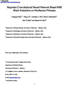
A deterministic chaotic system can be defined using the equation of the form of Xt+1 = BXt (1 − Xt ) where Xt and Xt+1 are, respectively, the previous and the future values of the generating process. B is a coefficient (control parameter) whose value can be generated between 0 and 4 to represent the complex system. The Logistic map represents deterministic system, which tends to evolve towards a well behaved chaotic “attractor”. The nature of chaotic dynamics depends on the complexity of system’s evolution and its dimension (Fig. 1a).
www.nonlin-processes-geophys.net/18/515/2011/
R. K. Tiwari and S. Maiti: Bayesian neural network modeling
517 Xt depends partly on the Xt−1 and partly on the random distributionεt . A 3-D phase-space characteristic is a plot of current observations X(t) on the X-axis, X(t + 1) on the Yaxis and X(t + 2) on the Z-axis. AR (1) model exhibits the tendency to cluster towards low values (Fig. 1b). 1.2.3
White noise
A white noise process is a fully uncorrelated system and therefore, these data scatter randomly across the entire phasespace. A 3-D phase-plot of such data is displayed in Fig. 1c for comparisons with the similar plots of chaotic, autoregressive and actual temperature data respectively shown in Fig. 1a, b and d. Apparently random data shows entirely different characteristics than the chaotic, autoregressive and the non-random temperature data. 2
Material and methods
2.1 2.1.1
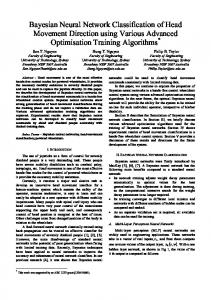
Fig. 1. (a–c) show phase diagram of non-stationary, nonlinear and random characteristics of different types of synthetic time series, respectively. (d) 3-D scatter plot of actual tree-ring temperature time series. The data characteristics apparently show that the temperature record is non stationary (between stochastic and chaotic).
Bayesian approach to temperature modeling Multi-Layer Perceptrons (MLP)
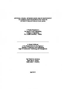
Multi-layer Perceptrons (MLPs) networks are parallel computational units composed of many simple processing elements which mimic the biological neurons (Fig. 2). The processing elements/nodes are interconnected layer by layer and the function of an each node is determined by the connections weights, biases and the structure of the network (Bishop, 1995; Poulton, 2001). Detailed sequential developments of the ANN methods are available elsewhere (Poulton, 2001; Maiti et al., 2007; Maiti and Tiwari, 2010b). In the popular back-propagation method, an error is usually minimized by adjusting weights and biases via the gradient based iterative chain rule from the output layer to the input layer (Rumelhart et al., 1986). Here in order to obtain global minimum, we use an optimization scheme which is based on the HMC simulations (also well known as leap-frog discretizations scheme) in conjunction with the Bayesian probability theory (Bishop, 1995; Nabney, 2004). We represent a geophysical observation through the following forward model: x = f (d) + ε
1.2.2
First order auto-regressive/AR (1) model
A first order autoregressive AR (1) model (Fuller, 1976) can be defined using the equation of the form of Xt = AXt−1 + εt ; where t = 1,2,3,.............N denotes the discrete time increment, A is a constant which can be estimated using the maximum likelihood method. Lag one autocorrelation coefficient describes the degree of signal correlation in the noise and is calculated from the data. If |A|=1, then the model reduces to random walk model; however, when |A| < 1, then it can be shown that the process is stationary. The parameter εt represents a purely random process (normal Gaussian), www.nonlin-processes-geophys.net/18/515/2011/
(1)
where f is a nonlinear function relating the model space and the data space, ε is the error vector, x is the data vector and d is the model vector. Commonly inversion of model d in Eq. (1) is performed via an iterative least square method. However this does not provide uncertainty measures, which are very essential for reliable interpretation of geophysical observations (Tarantola, 1987). For solving the Eq. (1) in the Bayesian sense, sufficient representative realizations (model/data pairs) from a finite data set s = {xk ,dk }N k=1 are considered. We can write the following equation as (Bishop, 1995; Nabney, 2004) d = fNN (x;w)
(2)
Nonlin. Processes Geophys., 18, 515–528, 2011
518
R. K. Tiwari and S. Maiti: Bayesian neural network modeling
Fig. 2. Schematic diagram of Multi-Layer Perceptron (MLP). Information flows from input to output layer through connection (synaptic weight). Weighted sum is passed through nonlinear activation function. Nodes are interconnected to the nodes at the next layer.
where d is the desired model, fNN is the output predicted by the network and w is the network weight parameter. In a conventional ANN approach, an error function ES = N 1P {dk − ok (xk ;wk )}2 is measured where dk and ok are, re2 k
spectively, the target/desired and the actual output at each node in the output layer. The error function is measured to know how close the network output o(x;w) is to the desired model d from the finite data set s = {xk ,dk }N k=1 . One can include regularization term to modify the misfit function, E(w) = µES + λER where, ER =
1 2
R P i=1
(3)
wi2 and R is total number of weights and
biases in the network. λ, µ are two controlling parameters known as hyper-parameters. The forward function used in each node is non-linear transfer function (tansigmoid) which facilitates to solve the non trivial problems. In the traditional approach, the training of a network starts with the initial set of weights and biases and end up with the single best set of weights and biases given the objective function is optimized. Nonlin. Processes Geophys., 18, 515–528, 2011
2.1.2
Developing the BNN algorithm for temperature record
Here in this scheme a suitable prior probability distribution P (w) of weights is considered, instead of a single set of weights. Following the Bayes’ rule, a posteriori probability distribution for the weights P (w|s) can be given as follow (Bishop, 1995; Khan and Coulibaly, 2006), P (w|s) =
P (s|w)P (w) P (s)
(4)
where P (s|w) and P (s) are the data set likelihood function and the normalization factor, respectively. Since the denominator P (s) in the above equation is inflexible, a direct inference of a posteriori P (w|s) is impossible. The probability distribution of outputs following the rules of conditional probability for a given input vector x can be given in the form (Bishop 1995; Khan and Coulibaly, 2006), Z P (d|x,s) = P (d|x,w)P (w|s)dw (5) www.nonlin-processes-geophys.net/18/515/2011/
R. K. Tiwari and S. Maiti: Bayesian neural network modeling Markov Chain Monte Carlo (MCMC) sampling plays a central role for evaluating posterior integrals. Accordingly the Eq. (5) can be approximated as P (d|x,s) =
N 1X P (d|x,wm ) N n=1
(6)
Where {wm } represents a MCMC sample of weight vectors obtained from the probability distribution P (w|s), N is the number of points and w sampled from. 2.1.3
Hybrid Monte Carlo algorithm (HMCA)
HMCA is used for updating each trajectory by approximating the Hamiltonian differential equations. HMCA uses Markov Chain Monte Carlo (MCMC) algorithm to draw an independent and identically distributed (i.i.d) sample {w(i) ;i = 1,2,....,N} from the target probability distribution P (w|s) (Metropolis et al., 1953; Hastings, 1970; Bishop, 1995). This is done to incorporate information about the gradient of target distribution and thereby it improves mixing in high dimension (see Duane et al., 1987; Andrieu et al., 2003). Markov process forms a sequence of “state” to draw samples from posterior probability distribution. The states are represented by a particle in the high dimensional network parameter space whose positions are defined by q ∈ R w . The Eq. (4) can be written in the form of π(q) ∝ exp{−E(q)} where π is a generic symbol and E(q) is a potential energy function for optimization problem (Duane et al., 1987). As suggested by Neal (1993) and further discussed by Bishop (1995) introducing momentum variables p with i.i.d standard Gaussian N P distributions, one could add a kinetic term V (p) = 21 pi2 to i=1
the potential term to produce full Hamiltonian (energy) function. This could be efficiently used to explore the large region of phase-space by simulating the Hamiltonian dynamics in fictitious time. Hamiltonian energy function on a fictitious phase space is given by (Duane et al., 1987; Neal, 1993), H (q,p) = E(q) + V (p)
(7)
The following equation represents the canonical distribution of Hamiltonian π(q,p) =
1 exp{−H (q,p)} QH
(8)
Here, π is a generic symbol, q is position and p is momentum. To discretize the equations of motion of particle, we employ the Metropolis algorithm following Neal (1993) and the leapfrog discretization scheme to explore the full phase space (q,p) without destroying time reversibility and volume preservations. To simulate the dynamics forward or backward in time τ , we first appropriately decide the step size θ and the number of iterations L and then consider the following sequence of steps for further computations. www.nonlin-processes-geophys.net/18/515/2011/
519 i. Randomly chose a direction α for the trajectory (Neal 1993; Bishop, 1995) in either +1 or −1 representing respectively forward and backward trajectory with the probability 0.5. The transition probability between qj and qi be the same at all times and each pairs of points maintain a mutual equilibrium. ii. The iterations start with the current state [q,p] = [(q(0),p(0)] of energy H (Metropolis et al., 1953; Hastings, 1970; Duane et al., 1987; Neal, 1993; Bishop, 1995). The momentum term p is randomly evaluated at each step. The algorithm carries out L steps with a step size of θ resulting in the candidate state, [w ∗ ,p∗ ] with energy H ∗ (Duane et al., 1987). iii. The candidate state may be either accepted or rejected according to Metropolis theory. The candidate state is accepted with usual Metropolis probability of acceptance,min{1,exp[−(H ∗ − H )]}, where H (.) is the Hamiltonian energy (Metropolis et al., 1953; Hastings, 1970; Duane et al., 1987; Neal, 1993; Bishop, 1995). If the candidate state is rejected then the new state will be the old state. In this way the summation of Eq. (6) is carried out to estimate the posterior probability distribution and thus allowing the optimization of the network (Neal, 1993). 2.1.4
General methodology
We consider a time series in the form of In the time series fore{x(1),x(2).................x(p)}. casting, ANN model is developed to learn a relationship between the current times series value with the past series value. Modeling /predicting the tree-ring temperature series is done to set up a relationship between a tree-ring temperature anomaly value, say x(n + p), and its previous series, x(n + p − 1),x(n + p − 2),.......x(p), as f : R n → R 1 ;x(n + p) = f {x(n + p − 1),x(n + p − 2),............x(p)}; (p = 1,2,......n), where x is variable; n is sample number used to construct the model (Zhang et al., 1998). The objective of the study in this paper is to derive the nature of f from the available time series data {x}N t=1 . In general, the function f is nonlinear and determined by ANN structure. If the nature of the time series is fully deterministic, then its behavior is predictable. However if the nature of the time series is random, then the prediction is impossible. The general procedure of the Bayesian neural network based algorithm for time series modeling is described as follows: Step 1: The data are pre-processed to scale the input/output series in between [−1 +1] so that the network can perform nonlinear mapping within the bound. It is important to arrange the input and corresponding data pairs in such a way that the network can learn from the training pairs (input/output) for desired step prediction. Nonlin. Processes Geophys., 18, 515–528, 2011
520
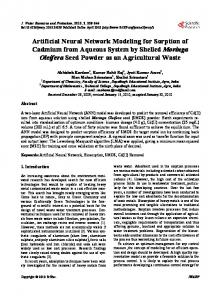
R. K. Tiwari and S. Maiti: Bayesian neural network modeling Step 2: Using the preprocessed data, a suitable prior distribution for weights and biases of the network is chosen. Step 3: A noise model is defined and a likelihood function is derived thereon. Step 4: Following the Bayes’ theorem, an expression for the posterior distribution of the weights is developed. Step 5: Step size, iteration number, simulation directions etc are set up for starting the hybrid Monte Carlo learning. Step 6: In the simulation a candidate state is accepted or rejected according to the Metropolis acceptance rule. Thereby most probable samples are chosen in order to maximize the posterior probability distribution and to evaluate the posterior integrals. Step 7: Post-process the predicted data to transform in original scale. If the optimization satisfies the goal in terms of error tolerance in data sets of validation and testing then stop the program and exit otherwise resume the process from the step 1. The flow chart of the methodology is given in Fig. 3.
2.2
Quantitative evaluation of models and comparison with tree-ring temperature record
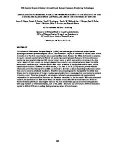
Before applying the above algorithm to the tree ring temperature record, we tested the method on synthetic time series generated from the AR (1) and chaotic models and the white noise data as described in Sect. 1.2 for different values of coefficients B and control parameter A. This experiment is actually done to test the authenticity and the predictive skill of the developed algorithm on simple known empirical models. For modeling we considered 256 data point out of which 50 % was used for training and remaining data for validation and testing. A fourth data set is also prepared by combing the above three basic time series, to represent the complex time series. Figure 4a–d shows the Pearson’s correlation coefficients between the actual and predicted data using the Bayesian neural network for all four time series. Following Mihalakakou et al. (1998) the predicted output value is appended in the input data base to predict next each step ahead. The BNN shows comparatively better prediction for the chaotic time series than the autoregressive (1) time series (Fig. 4a, b). As expected the Pearson’s correlation coefficient for the actual random data and the predicted data is almost negligible (Fig. 4c). The network shows average prediction for the mixed/pooled time series data (Fig. 4d). Obviously this experiment demonstrates the predictive skill of algorithm on the different types of time series irrespective of scale-unit. After a successful testing of the BNN algorithm on complex synthetic time series, we demonstrate the applicability of the Nonlin. Processes Geophys., 18, 515–528, 2011
Fig. 3. Flow chart of the general methodology.
proposed method on the newly constructed tree-ring temperature records over the Western Himalayas, India (Fig. 5). 2.3
Source and characteristics of tree-ring temperature record
A detailed description of analyzed tree-rings temperature variation record (Fig. 5) is discussed elsewhere (Yadav et al., 2004). Accordingly the natural and undisturbed open stands of Cedrus deodara (Roxb. Ex Lambert) G. Don at different localities in Uttarkashi and Chamoli in Uttaranchal, India, where healthy trees were growing on rocky hill slopes, was selected for the reconstruction of the time series. Samples were collected from “15 sites the form of increment cores with open stands” of Cedrus deodara. According to these authors at least two cores from each tree were taken at breast height (1.4 m) of the stem. The ring-widths of dated samples were evaluated against the chronologies created by visually assigning years to rings with different widths to 0.01 mm accuracy using the computer program COFECHA (Holmes, www.nonlin-processes-geophys.net/18/515/2011/
R. K. Tiwari and S. Maiti: Bayesian neural network modeling
521
Fig. 5. Tree-ring temperature variability time series from the Western Himalayas.
1983). Ring-width measurements series were standardized using the computer program ARSTAN (Cook, 1985). There are several reasons to focus on the tree-ring data of the Western Himalayas. Previous studies have shown that the tree-ring growth is highly sensitive to the variations of summer temperature. Consequently, these tree-ring chronologies have served as a proxy record for several paleotemperature reconstructions and these reconstructions have played vital role in assessing the reliability of solar and volcanic forcing on regional and hemispheric climate variations over the past centuries (Cook, 1985; Woodhouse, 1999; D’Odorico et al., 2000; Briffa et al., 2001, Cook et al., 2003; Jones and Mann, 2004; Boreux et al., 2009; Helama et al., 2009). Figure 5 exhibits a complex response of inter-decadal and inter annual pre-monsoon temperature variability for the last 774 yr. Several regional and global cooling and warming episodes match with the temperature variation (Yadav et al., 2004) attesting its global significance. This implies that the reconstructed tree ring temperature variation record (Yadav et al., 2004) analyzed here has been placed aptly both in global and regional context. Visual inspection of the temperature record exhibits distinct non-random noisy pattern with some significant oscillations (Tiwari and Srilakshmi, 2009). 2.4
Fig. 4. (a) Plot of prediction time ahead and correlation coefficient of theoretical chaotic time series with different Maximum Likelihood Estimator (MLE) values. (b) Stochastic time series (controlling parameter coefficient in a range of 3.5–4.0) (c) plot of prediction time ahead and correlation coefficient of random time series where mean = 0; standard deviation (STD = 1) (d) combined time series; random series (mean = 0; STD = 1) ;stochastic(Maximum Likelihood Estimator (MLE) constant = 0.5) and chaotic (controlling parameter constant = 3.8).
www.nonlin-processes-geophys.net/18/515/2011/
Parameterization and measures of model performance
It is essential to select an appropriate architecture of the network for modeling as to neural networks are generally sensitive to the number of neurons in their hidden layers. Several studies have shown that too few neurons in the hidden layer can lead to under fitting, while too many neurons in the hidden layer can also contribute to over fitting, in which all the training points are got well fit, but the fitting curves take wild oscillations between these points (Mihalakakou et al., 1998; Van der Bann and Jutten, 2000; Maiti and Tiwari, 2010b). During our experiment for searching an appropriate architecture, many network structures were tested (e.g. number of Nonlin. Processes Geophys., 18, 515–528, 2011
522
R. K. Tiwari and S. Maiti: Bayesian neural network modeling
Fig. 6. Errors in the prediction of the system with different network architectures for synthetically generated chaotic (B = 3.8), autoregressive (A = 0.5) and random model (a) errors of predictions of the system with different number of input nodes. (b) Errors of the system with different numbers of hidden layer node.
input nodes were taken from 1–50, number of hidden nodes were taken from 2–50) and errors were calculated for different architectures. Figure 6 shows the variations of prediction error, which is defined as an absolute difference between the observed and the predicted values with different input and hidden layers nodes. Figure 6 suggests that the best topology should consist of an input layer of having 5 nodes and a hidden layer of having 25 nodes. Following Nabney (2004), we also appropriately chose the initial prior hyper-parameters value λ = 0.01 and µ = 50.0. Since the Gaussian approximation to the weight posterior depends on being at a minimum of the error function (Nabney, 2004), we chose a very low tolerance value (10−7 ) for the weight optimization. 2.5
“One-lag” predictions
The procedure for one lag prediction is as follows (Mihalakokou et al., 1998): the BNN is trained over a certain part of tree-ring temperature data series, and subsequently validated and tested over the remaining parts of the data series. The network is used primarily for “one-lag” predictions, where the prediction of future values is based only on past observed values. For example, we consider a time series which is represented as x(ti ) where i = 1,2,....,N . For the first set of 5 inputs say {x(1),x(2),x(3),................,x(5)}, we predict the sixth value at x6 . Similarly, for the second set Nonlin. Processes Geophys., 18, 515–528, 2011
Fig. 7. One lag temperature anomaly reconstruction in the period (AD 1400–1600) using (a) artificial neural network (ANN) (b) Bayesian neural network (BNN) (c) BNN with confidence level (CL) of 95 %.
we take inputs as {x(2),x(3),................,x(6)} and predict the seventh value at x7 and so on. Training continues over all the training pair (Figs. 7–10). The same data base is also used for the conventional artificial neural network method and the autoregressive linear method as discussed above and the predicted values are compared with the actual tree-ring records for training, validation and testing (see Table 1). The comparative results are presented in Table 1 from which it can be seen that the HMC-based Bayesian neural network approach provides better predictive skill than both the ANN and the linear AR model. Figures 7 and 8 show the result for one lag prediction of ANN and BNN in the period 1400–1600 AD and 1800–2000 AD, respectively.
www.nonlin-processes-geophys.net/18/515/2011/
R. K. Tiwari and S. Maiti: Bayesian neural network modeling
523
Fig. 8. One lag temperature anomaly reconstruction in the period (AD 1800–2000) using (a) artificial neural network (b) Bayesian neural network(BNN) (c) BNN with confidence level (CL) of 95 %.
Fig. 9. One lag temperature anomaly reconstruction using Bayesian neural network in the period (a) AD 1232–1488, (b) AD 1489– 1745, (c) AD 1746–2000.
2.6
multi-step ahead prediction. However the accuracy is relatively less than the one-lag prediction because every time the predicted value rather than observed value appended in the input for future prediction. The standard deviation (STD) of the predictive distribution for the target d (see Eq. 6) can be interpreted as an error bar on the mean value o(x;wm ) (Figs. 7c and 8c). This error bar represents contribution from two sources, one is from the intrinsic noise on the target data and other one is from the width of the posterior distribution of the network weights (see flow chart). The 95 % confidence interval of the mean network o(x;wm ) has been estimated by adding and subtracting STD from o(x;wm ) following Nabney (2004).
“Multi-lag” predictions
For “multi-lag prediction”, a value is predicted one step into the future and then this predicted value is used as one of the lagged inputs for the next prediction of two time steps into the future (Mihalakokou et al., 1998): similarly, the predicted values at this second time step as well as the previous time step are used as lagged inputs for the next prediction of three time steps into the future. In this way, new predicted value is included in the input network database and is used to predict the future values. For instance, if the network is used to predict the sixth value x6 from the measured series x(1)..........,x(5), then the next neural network prediction x7 is made using as inputs x(2)..........,x(5) and x6 and the subsequent network prediction x8 is made using the time series values, x(3),x(4).........,x(5),x6 and x7 . In the beginning five measured values are used as inputs for the first prediction. Furthermore, it has been found that more the data are appended as inputs for the first output, longer the predictions span (Mihalakokou et al., 1998). This is useful for www.nonlin-processes-geophys.net/18/515/2011/
2.7
Application to tree-ring temperature record
Of the total 774 yr long tree-ring temperature data spanning over the period of 1226 AD–2000 AD, the first segment comprising of 1226 AD–1488 AD is used for the network training; the second segment spanning over 1489–1745 AD is Nonlin. Processes Geophys., 18, 515–528, 2011
524
R. K. Tiwari and S. Maiti: Bayesian neural network modeling Table 1. Model comparison statistics for training period (AD 1226– 1488) (subscript tr) and validation period (AD 1489–1745) (subscripted val) and testing period (AD 1746–2000) (subscripted tst). RMSE = root mean square error; RE = reduction of error statistics; d = index of agreement. Statistics Meantr Meanval Meanttst Standard deviationtr Standard deviationval Standard deviationtst RMSEtr RMSEval RMSEtst REtr REval REtst dtr dval dtst
3 3.1
Fig. 10. One lag temperature anomaly reconstruction using Artificial neural network in the period (a) AD 1232–1488, (b) AD 1489– 1745, (c) AD 1746–2000.
used for validating the network and the last segment from 1746 to 2000 AD is used for testing the network. After successful training, validation and testing the network, the results are presented in figures (Figs. 9 and 10). For reverse reconstruction the neural network based reconstruction is employed from the most recent tree-ring temperature anomaly value to the most past tree-ring temperature anomaly value up to AD 1226. It has been found that reconstruction based on the BNN methods from the present to the past is better than from the past to the present since the tree-ring temperature data from AD 1901 to 2000 were actually observed, the temperature anomalies before this are reconstructed (Yadav et al., 2004).
Observed Value
ANN
BNN
AR(1)
0.05 0.01 0.05 0.48 0.59 0.60
0.045 0.01 0.05 0.33 0.37 0.34 0.40 0.45 0.46 0.31 0.41 0.42 0.62 0.61 0.55
0.05 0.06 0.06 0.40 0.43 0.44 0.34 0.35 0.39 0.50 0.63 0.58 0.81 0.83 0.80
0.01 0.03 0.04 0.45 0.47 0.51 0.94 0.93 1.00 0.14 0.23 0.22 0.07 0.04 0.05
Results and discussions Comparison and statistical evaluation of predicted temperature and actualtree-ring temperature records
We have compared the present Bayesian neural network (BNN) results with the conventional neural network approach and the traditional statistical linear AR model. We have used the identical network structures for both the ANN and the BNN modeling. We have used scaled conjugate gradient (SCG) algorithm (Bishop, 1995; Van der Bann and Jutten, 2000), for the optimization process, which avoids the expensive line-search procedure of the conventional conjugate gradient technique. Experiments have shown that this is an efficient algorithm outperforming both the conjugate gradients and the quasi-Newton algorithms (Nabney, 2004). The network is optimized in 500 iteration/cycles with mean square error reaching up to 0.019. The standard AR model used in the present study is a special case of autoregressive moving average with an exogenous signal (ARMAX) model (Mihalakakou et al., 1998). In the AR model the present output signal say n P yp {k} = − a(i)y(k − i), where a = constant, is estimated i=1
as a linear combination of the fixed number of past inputs samples with (k = 0,1,2,3,4,..................) (Mihalakakou et al., 1998). yp {k} is scalar output signal at time tk = kτ (τ ) is a sampling period and k is the time index or the cycle number. p stands for prediction. Nonlin. Processes Geophys., 18, 515–528, 2011
www.nonlin-processes-geophys.net/18/515/2011/
R. K. Tiwari and S. Maiti: Bayesian neural network modeling
Fig. 11. Tree-ring temperature anomaly reconstruction using Autoregressive method (1) in the period (a) AD 1232–1488, (b) AD 1489–1745, (c) AD 1746–2000.
Comparison and correlation analysis between the actual and the predicted data shows that most of the predicted/reconstructed data points lie within the error bar and match well with the actual data points (Figs. 7c, 8c and 12c). Comparison of the BNN with the ANN and the AR (1) results suggests that the BNN shows a better predictive skill than the ANN and the AR (1) (Figs. 9–11). It may be noted that the results we have presented here are the mean of several hybrid Monte Carlo based simulation i.e. ensemble mean of more than 1000 simulations. We have further analyzed the result using different statistical measures. Statistical results show that the BNN performs generally better than the ANN and the AR (1) model (Figs. 8–12). The mean value and the standard deviation are quite consistent at some places, duplicative in training, validation and test period (Table 1). The root mean square error (RMSE) is a measure of error or the difference between observed (Oi ) and predicted(Pi ) by the model for sample N and is defined by (Woodhouse, 1999)
525
Fig. 12. The linear regression analysis of predicted value in the test period (1489 AD–2000 AD) by (a) autoregressive method (1), (b) artificial neural network, (c) Bayesian neural network.
RMSE =
v u N uP u (Oi − Pi ) t i=1 N
The RMSE indicates that the BNN model perform well than the ANN and the AR (1) model in the training, validation and the test period (smaller RMSE) (Figs. 8–12, Table 1). The two quantities RE (reduction of error) and the “d” (index of agreement) in Eqs. (10) and (11) are, respectively, the measures of the predictive ability of the models. Any positive value indicates that the reconstruction has some predictive skill. N P
RE = 1.0 −
(Oi − Pi )2
i N P i
www.nonlin-processes-geophys.net/18/515/2011/
(9)
(10) Oi2
Nonlin. Processes Geophys., 18, 515–528, 2011
526
R. K. Tiwari and S. Maiti: Bayesian neural network modeling
The RE values for all the three models are positive, but the RE for the BNN is higher than the ANN and the AR (1). The index of agreement d is suggested by Willmott (1981) as N P
d = 1.0 −
(Oi − Pi )2
i N P
(11)
[|Pi − O| + |Oi − O|]2
i
where d range from 0 to 1 with a value of 1 indicating a perfect association .The d statistic specifies the degree to which the observed deviations about the observed mean in magnitude and sign correspond to the predicted/reconstructed deviations about the observed mean. This also reflects sensitivity to both the differences in observed and predicted means and changes in proportionality (Willmott, 1981). All two d values of the BNN and the ANN may be considered good for validation and test period. Results also indicate that the BNN model slightly outperforms the ANN. Correlation analysis between the predicted temperature variability and the actual tree-ring temperature records suggests that the new HMC- based BNN result is consistent with high correlation coefficient ∼0.77 (Fig. 12c). It can be seen from Table 1 and Fig. 12 that the HMC- based BNN algorithm makes clearly better predictions than those of ANN and AR model in test period. Better predictive skills of the BNN methods than the other two approaches suggest that the method can be used for better prediction not only for climate/temperature records but also for other environmental data. We reiterate the fact that the BNN possess more mathematical soundness to give reliable prediction even if the data is tamed by some amount of correlated noise (Maiti and Tiwari, 2009, 2010b). There are many advantage of the BNN over the ANN. It takes care of the uncertainty of mapping from one domain to another in a natural way and thereby allows for measuring the uncertainty in prediction. Furthermore, the method is naturally parsimonious to prevent overfitting which is a very common ailment in any non-Bayesian ANN modeling. If size of the available data set is less, then the BNN does not necessarily need to reserve part of the data set for validation and testing (Bishop, 1995). The only disadvantage of the BNN methods is that it takes relatively more time to optimize the process since the relatively more parameters need estimation in the training process. The predicted result in the Bayesian frame work is reliable and does not involve any over and under fitting of data and hence more appropriate method to compare the previous results. 3.2
Physical significance and limitations
The reconstructed temperature variation record shows higher variability during the recent past since 16th century of the record as compared to the earlier part of the time series i.e. (AD 1226–1500). The reconstructed BNN temperatures record also exhibits unstable climate during the little ice age Nonlin. Processes Geophys., 18, 515–528, 2011
(LIA) (Bracuning, 2001; Zhang and Crowley; 1989; Yadav et al., 2004). Further cooling and warming trend of the reconstructed variability are also matching more or less with various regional climate variability of Asian monsoon region as reported by several workers (Briffa et al., 2001; Esper et al., 2002; Cook et al., 2003). The BNN modeling of the underlying temperature data presented here elucidate some better picture of the inherent trend in the data and its predictive nature. However there are some limitations too in the present modeling approach, which needs to be clarified here. The BNN model utilized in the present work is based on the assumption that the temperature/ring-width relationshiois remains stationary over this time. This, however, requires that potential covariates, such as precipitation, also remain stationary over the same time, which is not true. This implies that the underlying temperature time series is nonlinear and nonstationry in nature. In view of the above, it is somewhat difficult to conclude, at this stage, that the reconstructed/predicted record using the underlying technique would provide unique result for the detailed physical discussion. However the BNN model shows comparatively better results than the results of other two methods, particularly in this analysis as also demonstrated in theoretical applications. We also note here that the present predicted result is based on data driven approach without portraying any real physical processes involved in the variability of temperature and hence it is not prudent to conjecture or evoke any physical mechanism here. Based on the above statistical evaluations we may, however, argue that the present model reveal some deterministic pattern for the temperature variability, although it does not elucidate what are the possible sources that are actually involved in driving these distinct variability. We further note that our predictive analysis of synthetic data generated by three empirical models clearly distinguishes random and non-random pattern inherited in the data structures. Hence based on the best fit between the predicted model and the actual data, we may conjecture that the source of this variability could possibly emanate from some non-random processes, which is also evident in the spectra of the temperature records (Tiwari and Srilakshmi, 2009).
4
Conclusions
The present research suggests the use of BNN approach as a viable tool for modeling the tree ring temperature variation data. Its nonlinear character and capability to work with data make this method particularly appealing for application to extreme temperature variability. The robustness of BNN method is first demonstrated on the synthetic data generated by the well known empirical models and then applied to the Western Himalayas temperature variation records. Our analysis provides an instance of the quality of the fitness of BNN construction to the observed temperature data in comparison www.nonlin-processes-geophys.net/18/515/2011/
R. K. Tiwari and S. Maiti: Bayesian neural network modeling to the traditional techniques. Even with meager insight of the physical processes or the dynamics underlying the characteristics of the present and the past temperature variability, the BNN approach improves the prediction and could lead a better understanding of the basic phenomena. The underlying BNN approach would not only complement currents methods being used for prediction but would also help for understanding and measuring the uncertainty in network prediction take place due to the limited and the sparse density data. Inference is provided by an MCMC algorithm which provides a natural method for estimating uncertainty. It may be mentioned here that dendroclimate signals commonly become noisier/corrupted due to population dynamics, which most likely complicate the tree rings growth – temperature/climate relationships (Helama et al., 2009). The present results show that even over an intricate situation Bayesian ANN technique resolves considerably good temperature signals. Acknowledgements. We are indeed indebted to the unanimous reviewers for their very thoughtful review and invaluable suggestions to improve the manuscript and the associated editor for his encouragement. We are also extremely grateful to R. R. Yadav for providing his published tree-ring temperature data. We are also grateful to the Director NGRI for his permission to publish this work. Edited by: J. Kurths Reviewed by: two anonymous referees
References Andrieu, C., de Freitas, N., Doucet, A., and Jordan, M.: An introduction to MCMC for machine learning, Mach. Learn., 50, 5–43, 2003. Bishop, C. M.: Neural networks for pattern recognition, Oxford University Press, 1995. Blanco, J. A., Seely, B., Welham, C., Kimmins, J. P., and Seebacher, T. M.: Testing the performance of FORECAST, a forest ecosystem model, against 29 years of field data in a Pseudotsuga menziesii plantation, Can. J. Forest Res., 37, 1808–1820, 2007. Boreux, J.-J., Naveau, P., Guin, O., Perreault, L., and Bernier, J.: Extracting a common high frequency signal from Northern Quebec black spruce tree-rings with a Bayesian hierarchical model, Clim. Past, 5, 607–613, doi:10.5194/cp-5-607-2009, 2009. Bracuning, A.: Climate history of Tibetan Plateau during the last 1000 years derived from a network of juniper chronologies, Dendrochronologia, 19, 217–137, 2001. Briffa, K. R., Osborn, T. J., Schweingruber, F. H., Harris, I. C., Jones, P. D., Shiyatov, S. G., and Vaganov, E. A.: Low frequency temperature variations from northern tree ring density network, J. Geophys. Res., 106, 2929–2941, 2001. Cook, E. R.: A time series approach to tree-ring standardization, PhD Dissertation, Univ. of Arizona, Tucson, 1985. Cook, E. R., Krusic, P. J., and Jones, P. D.: Dendroclimatic signals in long tree-ring chronologies from the Himalayas of Nepal, Int. J. Climatol., 23, 707–732, 2003. Crowley, T. J.: Causes of climate change over the past 1000 years, Science 289(5477), 270–277, 2000.
www.nonlin-processes-geophys.net/18/515/2011/
527 D’Odorico, P., Revelli, R., and Ridolfi, L.: On the use of neural networks for dendroclimatic reconstructions, Geophys. Res. Lett., 27, 791–794, 2000. Duane, S., Kennedy, A. D., Pendleton, B., and Roweth, D.: Hybrid Monte Carlo, Phys. Lett. B, 195, 216–222, 1987. Esper, J., Schweingruber, F. H., and Winiger, M.: 1300 years of climatic history for western Central Asia inferred from tree rings, Holocene, 12, 267–277, 2002. Esper, J., Shiyatov, S. G., Mazepa, V. S., Wilson, R. J. S., Graybill, D. A., and Funkhouser, G.: Temperature sensitive Tien Shan tree ring chronologies show multi-centennial growth trends, Clim. Dynam., 21, 699–706, 2003. Fritts, H. C.: Bristtecone pine in the White Mountains of California; growth and ring-width characteristics. Papers of the laboratory of tree-ring research 4, University of Arizone Press, Tucson, 44 pp., 1969. Fritts, H. C.: Reconstructing large-scale climatic patterns from treering data, University of Arizona Press, Tucson, 567 pp., 1991. Fuller, W. A.: Introduction to the statistical time series, John Wiley and Sons, New York, 1976. Gramlich, L. G. and Brubaker L. B.: Reconstruction of annual temperature (1590–1979) for Longmire, Washington, derived tree rings, Quaternary Res., 25, 223–234, 1986. Hastings, W. K.: Monte Carlo sampling methods using Markov Chain and their applications, Biometrika, 57, 97–109, 1970. Helama, S., Makarenko, N. G., Karimova, L. M., Kruglun, O. A., Timonen, M., Holopainen, J., Meril¨ainen, J., and Eronen, M.: Dendroclimatic transfer functions revisited: Little Ice Age and Medieval Warm Period summer temperatures reconstructed using artificial neural networks and linear algorithms, Ann. Geophys., 27, 1097–1111, doi:10.5194/angeo-27-1097-2009, 2009. Holmes, R. L.: A computer-assisted quality control program, TreeRing Bulletin, 43, 69–78, 1983. Jones, P. D. and Mann, M. E.: Climate over past millennia, Rev. Geophys., 42(2), RG2002, doi:10.1029/2003RG000143, 2004. Khan, M. S. and Coulibaly, P.: Bayesian neural network for rainfall-runoff modeling, Water Resour. Res., 42, W07409, doi:10.1029/2005WR003971, 2006. Lindholm, M., Lehtonen, H., Kolstrom,T., Merilainen, J., Eronen, M., and Timonen, M. Climatic signals extracted from ring-width chronologies of Scots pine from the Northern, Middle and Southern parts of the boreal forest belt in Finland, Silva Fenn., 34, 317–329, 2000. May, R.: Simple mathematical models with very complicated dynamics, Nature, 261, 459–467, 1976. Metropolis, N., Rosenbluth, A. W., Rosenbluth, M. N., Teller, A. H., and Teller, E.: Equations of state calculations by fast computing machines, J. Chem. Phys., 21, 1087–1091, 1953. Maiti, S. and Tiwari, R. K.: A hybrid Monte Carlo method based artificial neural networks approach for rock boundaries identification: A case study from the KTB bore hole, Pure Appl. Geophys., 166, 2059–2090, doi:10.1007/s00024-009-0533-y, 2009. Maiti, S. and Tiwari, R. K. Automatic discriminations among geophysical signals via the Bayesian neural networks approach, Geophysics, 75(1) E67–E78, doi:10.1190/1.3298501, 2010a. Maiti, S. and Tiwari, R. K.: Neural network modeling and an uncertainty analysis in Bayesian framework: A case study from the KTB borehole site, J. Geophys. Res., 15, B10208, doi:10.1029/2010JB000864, 2010b.
Nonlin. Processes Geophys., 18, 515–528, 2011
528 Maiti, S., Tiwari, R. K., and Kuempel, H.-J.: Neural network modeling and classification of litho-facies using well log data: A case study from KTB borehole site, Geophys. J. Int., 169, 733–746, doi:10.1111/j.1365-246X.2007.03342.x, 2007. Mihalakakou, G., Santamouris, M., and Asimakopoulos, D.: Modeling ambient air temperature time series using neural networks, J. Geophys. Res., 103(D16), 19509–19517, 1998. Monge Sanz, B. M. and Medrano Marqu´es, N. J.: Total ozone time series analysis: a neural network model approach, Nonlin. Processes Geophys., 11, 683–689, doi:10.5194/npg-11-683-2004, 2004. Nabney, I. T.: Netlab Algorithms for pattern recognition, Springer, New York, 2004. Neal, R. M.: Bayesian learning for neural networks, SpringerVerlag, Inc., New York, 1993. Poulton, M.: Computational neural networks for geophysical data processing, Pergamon, 2001. Rumelhart, D. E., Hinton, G. E., and Williams, R. J.: Learning representations by back-propagating errors, Nature, 323, 533–536, 1986. Tarantola, A.: Inverse Problem Theory, Elsevier, New York, 1987.
Nonlin. Processes Geophys., 18, 515–528, 2011
R. K. Tiwari and S. Maiti: Bayesian neural network modeling Tiwari, R. K. and Srilakshmi, S.: Periodicities and Non-stationary modes in tree rings temperature variability record of the western Himalayas by multi-taper and wavelet spectral analyses, Curr. Sci. India, 97(5), 705–709, 2009. Van der Bann, M. and Jutten, C.: Neural networks in geophysical applications, Geophysics, 65, 1032–1047, 2000. Yadav, R. R., Park, W. K., Singh, J., and Dubey, B.: Do the western Himalayas defy global warming?, Geophys. Res. Lett., 31, 1–5, 2004. Zhang, J. and Crowley, T. J.: Historical climate records in China and reconstruction of past climates (1470–1970), J. Climate, 2, 833–849, 1989. Zhang, G., Patuwo, B. E., and Hu, M. Y.: Forecasting with artificial neural networks: The state of the art, Int. J. Forecast., 14, 35–62, 1998. Willmott, C. J.: On the validation of models, Phys. Geogr., 2, 184– 194, 1981. Woodhouse, C. A.: Artificial neural networks and dendroclimatic reconstructions: an example from the Front Range, Colorado, USA, Holocene 9, 521–529, 1999.
www.nonlin-processes-geophys.net/18/515/2011/