Bayesian Sequential Parameter Estimation by Cognitive Radar With

974

IEEE TRANSACTIONS ON SIGNAL PROCESSING, VOL. 63, NO. 4, FEBRUARY 15, 2015

Bayesian Sequential Parameter Estimation by Cognitive Radar With Multiantenna Arrays Anish Turlapaty, Student Member, IEEE, and Yuanwei Jin, Senior Member, IEEE

Abstract—In this paper we consider the problem of Bayesian sequential parameter estimation of extended targets for cognitive radar with multi-antenna arrays using adaptive waveforms. The target is modeled as a complex Gaussian random process. Using iterative waveform transmission, the cognitive radar estimates the target’s characteristic parameters and updates its probabilistic model based on new measurements. The adaptive waveform is designed by minimizing the conditional entropy from the posterior density of the model parameters. We analyze the performance of the developed Bayesian sequential estimation algorithm and derive expressions for the signal-to-noise ratio gain, the asymptotical posterior Cramer Rao bound, and the mutual information gain. The analysis and numerical simulations demonstrate that the adaptive sequential Bayesian estimator yields accelerated convergence of the estimate towards its true value and a smaller estimation error compared with the conventional Bayesian estimator that uses fixed waveform transmission under Gaussian or non-Gaussian noise. Index Terms—Bayesian sequential estimation, cognitive radar, multi-antenna array, waveform design.

I. INTRODUCTION

C

OGNITIVE radar is an emerging technology that aims to explore a higher level of sensing adaptation and biologically-inspired intelligence for modern radar design. It is generally believed that a cognitive radar comprises the processes of feedback, learning, information preservation, and adaptability in transmission [1], [2]. It adapts its transmission waveforms, radar beams, and other electronic, data processing capabilities in order to achieve superior performance in detection, estimation, and tracking by exploiting various knowledge sources. Extensive research has been conducted in the context of cognitive radar for the problems of target recognition [3], [4], tracking [5], [6] and other topics, which by no means is an exhaustive list of all the referencing. Different than the aforementioned work in cognitive radar, this paper aims to address the problem of Bayesian sequential Manuscript received March 20, 2014; revised October 20, 2014 and November 21, 2014; accepted December 19, 2014. Date of publication December 24, 2014; date of current version January 23, 2015. The associate editor coordinating the review of this manuscript and approving it for publication was Dr. Slawomir Stanczak. This work was supported in part by the U.S. Army Research Laboratory, the Office of Naval Research, and the Army Research Office under Grant W911NF-11-1-0160 and the National Science Foundation under Grant CMMI-1126008. The authors are with Department of Engineering and Aviation Sciences, University of Maryland Eastern Shore, Princess Anne, MD 21853 USA (e-mail: [email protected]; [email protected]). Color versions of one or more of the figures in this paper are available online at http://ieeexplore.ieee.org. Digital Object Identifier 10.1109/TSP.2014.2386292

estimation of statistical properties of radar targets by multi-antenna arrays. The estimation problem is studied under the cognitive radar framework: By adapting its transmission, a cognitive radar can influence its future measurement, which in turn enables efficient and accurate target parameter estimation in the Bayesian sense. Transmission waveform design is performed under the criterion of minimizing the conditional entropy of the posterior density of the target parameter. Hence, the Bayesian estimate, which is determined by the posterior density, converges faster to its true value compared to the case when nonadaptive equal power allocation waveform transmission or conditional mutual information based waveform is utilized. We call this process “cognitive” in that it resembles the perception-action cycle described by the Bayesian brain theory [7]–[9], which aims to minimize “uncertainty” (quantified by conditional entropy) in the cognitive system [10], i.e., the radar estimator in our case. On the other hand, from the Bayesian theory perspective, this paper shows that under Gaussian or non-Gaussian noise models, the use of adaptive transmission by multi-antenna arrays in the Bayesian sequential estimator yields accelerated convergence and improved estimation efficiency than the conventional non-adaptive Bayesian estimator or the adaptive estimator based on conditional mutual information waveforms. A. Conventional Bayesian Sequential Estimation (BSE) Bayesian estimation is an application of Bayesian decision theory where a parameter or a state vector is estimated based on available measurements. In its general form, let unknown paramebe the vector of ters with the prior probability density function and be the vector of observations dependant on the unknown parameters. Using the Bayes’ theorem for random variables , the posterior probability density is . This expression shows that the posterior beliefs of the unknown parameters can be modified by taking the observation data into account. Non-sequential (or batch) Bayesian estimation is well studied in literature (e.g., [11]) and is frequently used for estimating radar target response [12]. When this Bayesian process is done recursively in time with the incorporation of new measurements at each iteration, it is known as the Bayesian sequential estimation (BSE) [13]. The BSE method sequentially minimizes the Bayes risk or a loss function such as the estimation error (e.g., Bayesian mean squared error) and recursively updates the posterior probability density function (pdf) of the parameter given new measurements at each iteration. Sequential methods to calculate the posterior density become extremely important in pragmatic problems where implementation and speed are an issue. Bayesian sequential estimation is successfully used in

1053-587X © 2014 IEEE. Personal use is permitted, but republication/redistribution requires IEEE permission. See http://www.ieee.org/publications_standards/publications/rights/index.html for more information.

TURLAPATY AND JIN: BAYESIAN SEQUENTIAL PARAMETER ESTIMATION

wide range of disciplines. Some examples include sequential estimation of probability of detection for target tracking in sonar [14], passive source localization and weak signal detection [15], etc. However, the classic BSE method does not involve the study of the impact of transmission waveforms. B. Contribution of This Paper This paper develops Bayesian sequential estimation algorithms for extended radar targets using adaptive sensor arrays in a cognitive radar framework. The contribution of the paper can be characterized in the following perspectives. First, unlike conventional Bayesian sequential estimation problems that do not address the impact of adaptive waveform transmission on the estimator (e.g., [15], [16]), the focus of our problem is to examine the asymptotic efficiency, accuracy and computational complexity of the Bayesian sequential estimator with the aid of adaptive waveforms by a multi-antenna array radar. By examining the asymptotic Bayesian Cramer Rao bound and the error variance of the sequential estimator, we demonstrate that, by incorporating adaptive waveforms, the proposed scheme achieves accelerated convergence and improved estimation accuracy compared with the conventional Bayesian estimators. Second, the goal of the parameter estimation problem we consider is to extract the statistical properties of extended targets using antenna arrays. Since the relationship between the measurement and the unknown parameter is nonlinear, the waveform design problem is solved by minimizing the conditional entropy of posterior probability density of the unknown target parameter, which is equivalent to maximizing mutual information between the measurement and the unknown parameter directly. For comparison, we also consider the waveform design problem by maximizing the conditional mutual information between the measurement and the channel response which is a function of the unknown parameter. We show that the minimal conditional entropy method yields a slightly better estimation performance than the maximal conditional mutual information method under the Gaussian noise model. The difference is more pronounced when the noise is non-Gaussian (e.g., Laplacian noise [17]). Note that, adaptive waveform techniques for radar have been extensively studied (e.g., [3], [4], [12], [18]–[21]). The work in [3], [4] applies adaptive waveforms with Bayesian updates to cognitive radar to address the problems of classification and/or detection. The work in [12], [18]–[21] examines various radar waveform design criteria such as mutual information and minimum mean squared error, but not in the framework of Bayesian estimation. Different than these works, the waveform design problem we study in this paper is to improve the convergence and accuracy of target parameter estimation under the Bayesian sequential estimation framework. Furthermore, the problem of waveform design in frequency domain for sensing extended targets using information theory was discussed before (see e.g., [3], [18]). However, the design in [3], [18] is limited to a single antenna case and assumes full knowledge of the power spectral density of the target response. In our approach, we extend the design to multi-antenna arrays, thus, enabling the utilization of spatial diversity for waveform adaptation based on partial knowledge of the spatial covariance of the target response. Third, the proposed methodology of Bayesian estimation using adaptive waveforms can be applied to general target and

975

noise models. This is because the formulation of the posterior probability density function of the target parameters is generic and can be solved by numerical means for general statistical models other than Gaussian (see, e.g., Laplacian noise [17]). However, we show that computation can be considerably simplified when a Gaussian target model and a Gaussian noise model are adopted. The remainder of this paper is organized as follows. Section II presents the signal model and the Bayesian sequential estimation problem. Section III describes adaptive waveform design by minimum conditional entropy. Section IV presents the performance analysis. Section V presents the numerical simulation results. Conclusion is provided in Section VI. II. SIGNAL MODEL AND PROBLEM FORMULATION A. Signal Model We consider a wide-band multi-antenna radar system with an -element subarray and a -element subarray where both subarrays can transmit or receive. This is the case where the transmit and receive arrays use a single array. Extension to the case of separate arrays is straightforward and will not be discussed in this paper. The general setup for the cognitive radar is that, first, the subarray sends a probing signal to the field, the returned signals are received at the subarray . Based on the received signals, the characteristics of the scattering field is examined, and a new set of probe signals are emitted from subarray to the same scattering field. The returned backscattered signals are received for target parameter estimation and detection. The signal model consists of the array model and the radar scattering model. For the subarray , the transmit array is characterized by a sampled version of the array maniat the -th azimuth angle fold and the -th discrete frequency . We assume that the manifold is sampled well above the spatial and temporal Nyquist rates. As a rule of thumb, the number of frequencies , where BW is the system bandwidth and is coherence bandwidth of the channel [20], [22]. Simi. The larly, the receive array manifold is denoted by array manifold represents the response of the array to a unit energy scatterer corresponding in the azimuth-frequency domain. Consequently, the transmit and receive array manifold matrix is given by (1) (2) respectively. Similarly, we define the transmit array and receive array manifold matrix for subarray as follows, respectively, (3) (4) where and is the transmit array and receive array manifold at azimuth and frequency for the subarray , respectively. Next, let denote the complex radar return from the scatterers along azimuth direction . Thus, the target channel response at frequency is represented by the collection of returns from all the azimuth directions as follows, [21] (5)

976

IEEE TRANSACTIONS ON SIGNAL PROCESSING, VOL. 63, NO. 4, FEBRUARY 15, 2015

The vector (5) is considered as the azimuth angular distribution of the radar channel response of the scatterers in the radar field of view under a range cell (also see e.g., [23]–[25]). Note that the coefficients of the target impulse response (i.e., the time domain equivalent of by the inverse Fourier transform) are closely related to the target radar cross section (RCS) and are modeled as zero mean, finite covariance, wide sense stationary uncorrelated scattering (WSSUS) random processes in many wave propagation and radar literature [26]. The frequency domain characterization of the target, , can be derived by the Wiener-Khintchine theorem [20], [27]. Hence, we assume that target channel response is, in general, a zero mean complex random vector process (6) where is the probability density function conditioned on the parameter . Note that the expression in (6) is general and can be applied to Gaussian or non-Gaussian target models. Next, we assume that the frequency are sampled one coherence bandwidth apart. Hence the channel response vectors at different frequencies are considered to be independent. We denote the waveform that will be emitted from the sub-array at frequency as

In order to simplify the notation, we let denote the index of received data snapshots at the -th iteration in the -th cycle , which yields (13) Next, by grouping obtain

frequency components into vectors, we (14) (15) (16) (17)

and is a diagonal block matrix in the -th transmission cycle. Hence, the received signal over all the frequencies can be written as (18) and the parameter set to be estimated is . indicates that the channel is a function of parameter , which is typically nonlinear. Next, let denote the collection of measurements, the joint pdf at the -th iteration takes the form of (19)

(7) where the total transmission energy is Thus, the received scattered signal at sub-array A becomes

.

where rameter

denotes the prior probability density of the pa. Then, the posterior pdf at the -th iteration is

(8) where is the general noise vector with pdf is independent of the target response, i.e.,

(20)

and (9)

Here, the denominator is also called evidence (up-to the -th iteration) and is given by the integral of the numerator over . Next, we re-write (20) as a recursive posterior pdf

Next, we re-write (8) as

(21)

(10)

where the prior probability density available at the -th iteration is given by

where the waveform to be designed is

(22) (11)

is the array illumination vector where that depends on the array manifold and the transmission signal .

and the conditional density function in (21) is given by

(23)

B. The Bayesian Sequential Estimation Problem The sequential signal transmission and reception protocol can be described as follows. The protocol consists of two nested loops. The outer loop with index is named cycle; at the end of each cycle a new radar waveform is designed for the next cycle. Within each cycle, the new designed waveform is transmitted times to obtain data snapshots. Under this protocol, the signal model in (10) can be re-written as

where is the probability density of given and . Ideally, the posterior probability density function will show a sharp peak at the true value of , i.e., [11]. By the classic Bayesian estimation theory [28], the optimal estimate of is obtained in the sense that the Bayesian (posterior) mean square error (BMSE) is minimized, which yields

(12)

(24)

TURLAPATY AND JIN: BAYESIAN SEQUENTIAL PARAMETER ESTIMATION

where the posterior pdf is sequentially updated by (21) and (22). Next, the sequential estimation process will terminate when a stopping criterion is satisfied. Here we use the following stopping criterion

(25) where

and . Note that is the Fisher information (FI) of the posterior density defined in Section IV.C. The error variance term is (26)

Equation (25) implies that the stopping rule applies when the finite backward difference of deviation between the inverse of the averaged FI and the average error variance reaches a predetermined tolerance level . We choose this stopping rule (25) because it results in a monotonous decreasing function and is algorithm independent based on observations in our numerical simulation studies. The final estimate of the sought parameters are .

977

lihood is also complex Gaussian irrespective of the target model and prior probability density of , i.e., (29) Inserting (29) in (23) yields (27) For a general extended target model, for example, a mixed target model that includes mixtures of time varying Swerling targets of different kinds [30], [31], the function must be evaluated by numerical means. Remark 2 (Under Gaussian Target Channel Model): The solution to (24) is influenced by the underlying target channel model . In this paper, we consider a Gaussian target model. This is because it is not uncommon to adopt a Gaussian model for characterizing an extended target’s channel response (see, e.g., [19], [20]). Furthermore, the Gaussian assumption simplifies the computation of the posterior probability density of the target parameter. Hence, in this paper we assume the target channel response is a multivariate complex covariance Gaussian process with zero mean and an matrix , i.e., (30) where the covariance model for

is given by

C. Remarks on Models of Noise, Target, and Prior Density Equation (24) is generic and shows that the estimate depends on posterior density of the parameter . In general it must be calculated numerically irrespective of any assumptions regarding the noise and target model. However, simplification of calculation is possible under the Gaussian assumptions, as what is given in this paper, regarding the target channel model and the additive noise model. The following four remarks discuss the impact of the target model, the noise model, and the prior probability density. Remark 1 (Under Gaussian Noise Model): From (21), we see that the posterior density depends on the conditional likelihood function in (23), which in general has to be computed numerically. However, under the Gaussian noise model, a simplified expression of is obtained by the following proposition. Proposition 2.1: Given the signal model (13) and the Gaussian noise model , the conditional takes the form of likelihood function (27) where

is given by

(31)

where is the spatial spectral variance of the -th frequency channel, which is assumed to be known and normalized to unity for simplicity, i.e., . For brevity, in what follows, we let denote and use for scalar index and for matrix/ depends on the physical channel vector index. The value of parameters, such as angular spread for distributed sources [22], [24]. For a small angular spread, will be close to 1. As the will decrease to zero. The effecangular spread increases, tive rank of will vary from 1 to as decreases from 1 to 0. The motivation for the geometric sequence structure in terms of in (31) is that the signal correlation between closer angles is higher than those widely separated (see similar models in [32], [33]). We also allow negative value of to account for negatively correlated radar return signals [33]. This statistical model of the radar scattering return is often valid for characterizing extended targets using antenna arrays (see [34] for more complicated models). Hence, the -th entry is given by (32)

(28) Proof: The derivation of (27) follows [29] for conditional densities and is also similar to the Bayesian linear models in and the -th measurement is [28]. The joint pdf of given by . In this joint has to be condensity, the conditional likelihood of structed from the available probabilistic models of the target and the noise. Under the Gaussian noise model, the conditional like-

Under the Gaussian target and a non-Gaussian noise model, the expression (23) does not lead to the exponential structure given in (27). For example, one form of frequently encountered non-Gaussian noise is Laplacian noise (or called impulse noise) and is typically characterized as noise whose distribution has a “heavy tail” behavior (see e.g., [17]). The probability density function of complex Laplacian noise with a zero mean and standard deviation is given by, [35] (33) Hence, the integration in (23) does not lead to a separable functional structure as in (27). In this case, even for a Gaussian

978

IEEE TRANSACTIONS ON SIGNAL PROCESSING, VOL. 63, NO. 4, FEBRUARY 15, 2015

target, the likelihood function in (23), the posterior density in (21), and the posterior mean in (24) have to be evaluated using numerical integration. Remark 3 (Under Gaussian Target Channel Model and Gaussian Noise Model): The probability density function is Gaussian when both the target model and the noise model are assumed to be Gaussian. We have the following proposition. Proposition 2.2: Given the signal model (13), if both components and are complex normal processes, the marginal likelihood expression is a Gaussian probability density function, which takes the form of

III. ADAPTIVE WAVEFORM DESIGN Equation (24) reveals that the estimate is determined , which is also influenced by by the posterior pdf the waveform . The goal of waveform design is to change the posterior pdf by adapting the transmission waveforms so that the sequential estimation process reaches its optimal value with lesser number of measurements or iterations. A. Minimum Conditional Entropy (MCE) The approach is based on maximizing the mutual information between the parameter and the measurements defined by (40)

(34) where the conditional covariance matrix . Proof: Inserting the Gaussian target channel model (30) in (28) yields (35) where the inverse posterior covariance of

where the entropy of

is given by (41)

and the conditional entropy of defined as

given the measurements is (42)

is (36)

and the conditional mean (37) By (35), (27) can be re-written as

where the posterior pdf is given by (21). By (41) and (42), we rewrite (40) in terms of entropies. Since the first term in (40) is independent of , maximizing the mutual information becomes equivalent to minimizing the condi, tional entropy. Note that the total energy is but optimization can be performed at individual frequency separately for estimating individual parameter . Hence, the optimization problem at each frequency is formulated as

(43) (38) where (39) By the Woodbury’s matrix identity [36], the exponent term in (38) can be re-written as , which leads to (34) as the final likelihood function corresponding to Gaussian target and noise models. The pdf in (34) is a simplified form of (27). Note that in and in (23) are this case, a conjugate pair. The function in (27) reduces to a Gaussian structure in (35). Remark 4 (About Prior Probability Density Function): The computation in (24) also depends on the prior probability density , which is assumed to be non-informative, for example, a Gaussian or a uniform density. Our numerical simulations show that it is robust against the prior distribution. This is not surprising because the parameter to be estimated is a deterministic value and is modeled as a random variable under the Bayesian estimation framework. Under a large sample size, the impact of the choice of a non-informative prior probability density becomes negligible [11].

Note that earlier research reveals the relationship between the maximum mutual information (MI) and the minimum mean square error (MMSE). For instance, under Gaussian noise condition, the maximum of MI corresponds to lowest MMSE due to the linear relationship between the derivative of MI and the MMSE [37], [38]. Furthermore, an examination of the relationship between mutual information and the Bayesian decision theory reveals that the greater the mutual information between the parameter and its measurement, the better the expected performance in the best Bayes risk decision procedure, for example, Bayesian estimation [18], [39]. Hence, we conjecture that the MCE method is optimal in the sense that the waveform that maximizes the mutual information (MI) between the and the measurements would minimize the Bayesian mean square error (MMSE). Although no analytic result is provided due to the complexity of the problem, we rely on numerical means. In Section V.C we show by linear regression that there is a linear relation between conditional entropy and the base-2 logarithm of the posterior error variance under Gaussian or non-Gaussian noise models. The observation is motivated by the Shannon’s entropy inequality for differential entropy (i.e., continuous), [40] (44)

TURLAPATY AND JIN: BAYESIAN SEQUENTIAL PARAMETER ESTIMATION

TABLE I OUTLINE OF THE BAYESIAN SEQUENTIAL ESTIMATION ALGORITHM

979

surements and the target response rameter is defined by

given the pa-

(45) and its The first term in (45) is the entropy of pdf is given by (34). Note that (45) differs from (40) in that (45) is an indirect measure of the mutual information between the measurements and the unknown parameter through the target channel response, while (40) computes directly the mutual information between the measurements and the unknown parameter. A major advantage of the MCMI approach is that analytical expression for the waveform can be formed under Gaussian target and noise assumptions. Since both pdfs are Gaussian, (45) can be further simplified (by omitting the terms that are independent of ) as

(46) is unknown, we replace it with Furthermore, since with being the estimated value at the -th iteration. Hence, the optimization problem can be formulated as follows:

which becomes equality for Gaussian densities. Note that the parameter’s pdf approximates to a Gaussian density especially as the number of measurements increases (invoking the central limit theorem). Hence, the relation in (44) becomes equality which suggests a linear relation between entropy and the logarithm of error variance, which also implies that a waveform that minimizes the conditional entropy in (42) is the optimal waveform for estimation of the parameter. Hence, the proposed waveform design can be summarized in the following proposition. Proposition 3.1: Under the constant total energy constraint, for the linear radar signal model in (18), the sequential estimation process of the parameter defined in (6) can be accelthat minimizes the erated by designing a waveform conditional entropy of the posterior density of given measurements. Next, the optimization problem (43) is solved numerically using constrained nonlinear optimization. At each iteration the posterior pdf is numerically evaluated using (21). We then use the measurement from previous cycle and the waveform transmitted from previous cycle to initialize the numerical optimization algorithm. The optimization algorithm uses (42) to evaluate the entropy for each possible waveform structure. Specifically, we use active-set algorithm [41], [42] which is a quasi-Newton approach to determine the minimum of the conditional entropy. Finally, the Bayesian sequential estimation algorithm is summarized in Table I. B. Benchmark Approaches 1) Maximum Conditional Mutual Information (MCMI): In this approach, the conditional mutual information of the mea-

(47) Hence, the rationale for the MCMI waveform design can be summarized in the following proposition. Proposition 3.2: Under the constant energy constraint and the Gaussian assumptions, given a linear signal model with additive noise (18), the sequential estimation performance for the parameter can be accelerated by using an indirect tractable method, that recursively maximizes i.e., designing a waveform the conditional mutual information between the measurements and the target channel response which is a function of the parameter . Next, the solution to (47) for is calculated from a product of an orthogonal matrix, an energy allocation matrix and eigen vectors of the target covariance matrix as follows: (48) is a matrix with orthogonal vectors derived from , i.e., the columns of the matrix are the same as the singular vectors of the covariance matrix and the number of columns is equal to the rank of the covariance are eigen vectors of and matrix. is obtained by a water-filling type of algorithm (49)

where

where is the energy allocation factor in the -th dimension given by (80) The derivation of this waveform is provided in Appendix I. 2) Equal Power Allocation (EPA): In this algorithm we implement sequential Bayesian estimation without waveform adaptation. Here the same amount energy is transmitted in each of angles . The same waveform is transmitted

980

IEEE TRANSACTIONS ON SIGNAL PROCESSING, VOL. 63, NO. 4, FEBRUARY 15, 2015

repeatedly until the stop criterion is satisfied for the estimation process. C. Impact of Multi-Antenna Arrays The use of multi-antenna array enables a better spatial characterization of extended targets than that for a single antenna [43]. In this paper, the waveform design problems in (43) and (47) are solved by treating the transmit and receive array manifolds and the transmitting signals as coupled parameters, which gives rise to the illumination waveform . In real applicashould be generated to excite tions, the transmit signals the antennas before illumination. A close examination of (11) reveals that one possible solution is the least-squared solution

For EPA, the transmitting energy is equal in all directions, hence are orthogonal. This observation implies the columns of that the steering vectors should be chosen to be orthogonal. This requirement can be met in that for well separated azimuth angles (by one beamwidth), the steering vectors are approximately orthogonal [43]. Thus, for the non-adaptive method, if we choose and , the transmission waveform can be obtained straightforwardly once the array parameters are chosen. For the adaptive methods, energy allocation is determined by the water-filling algorithm based on the eigen values of the matrix at each transmission. The columns of are not orthogonal. The least squared solution for is usually can be neither optimal nor desirable. The signal vector obtained by solving an over-determined or under-determined system depending on the array manifolds. Other possible solutions include adaptive beamforming techniques for the transmitter array and the receiver array. For example, one can design a receive beamforming matrix adaptively by adjusting to minithe weights and the number of illumination angles mize . Due to space limitation, a more general treatment for array beampattern design and transmit waveform coding design will be presented elsewhere. IV. PERFORMANCE ANALYSIS We analyze the performance of the three different algorithms (MCE, EPA and MCMI). A. SNR Gain (SNRG) We define SNR gain for each channel at as the ratio of output SNR to input SNR as follows (see also [28]): (50) where the input SNR (ISNR) at is defined as,

under Gaussian noise model (51)

and the output SNR (OSNR) at

is defined by

using the eigen decomposition of the covariance matrix and also the decomposi, tion of the waveform we obtain OSNR(q) at the -th iteration

(53) Next we evaluate (53) for the methods EPA and MCMI. For MCE, we rely on numerical means. SNR Gain for EPA: For EPA the waveform does not change with iterations and given by . Thus, we have

(54) due to in this case. Hence (0 dB) which implies that the SNR gain is independent of and thus is not very useful for frequency allocation of energy. SNR Gain for MCMI: For MCMI, the waveform is adapted at the end of each cycle . As the estimate approaches the true value , (53) can be simplified as , which yields (55) The SNR gain is affected by the structures of the waveform matrix of the antenna array and the covariance matrix of the target response. By (89) and (90) in Appendix II, we obtain the lower bound and the upper bound as follows: (56) The maximum gain is achieved when all the energy is concentrated in the direction corresponding to maximum eigen value. The minimum gain corresponds to the case of equal energy allocation or when all eigen values are equal to 1. B. Mutual Information Gain (MIG) The gain in mutual information (or reduction of uncertainty) of the estimation process between the methods MCE and EPA is defined as the difference between the mutual information of the two methods. Consider and as the measurements in the MCE and EPA method, respectively. The mutual information gain at is defined by (57) By using the definition of mutual information the information gain can be expressed as the difference between corresponding conditional entropies, i.e.,

(52) The quantity SNR gain can be used to determine the channel condition for sequential estimating the unknown parameter and thus is very useful for allocation of energy in different frequencies, [4], [44]. By

(58) This difference basically quantifies the reduction in uncertainty (entropy) due to waveform adaptation and it is directly related to the improvement of accuracy as shown in Section V.C. Under

TURLAPATY AND JIN: BAYESIAN SEQUENTIAL PARAMETER ESTIMATION

Gaussian noise model, by the definition of the posterior probability in (20) and (42), as well as the prior , the conditional entropy by the MCE method becomes

981

Inserting (34) in (62) and ignoring the terms independent of yields

(59) Similarly, in the case of EPA method with non-adaptive waveforms, the conditional entropy is presented as (63)

(60) Both (59) and (60) are computed using numerical means over the posterior pdfs given in (20). C. Asymptotic Bayesian Cramer Rao Bound (BCRB) The Bayesian Cramer Rao bound (also known as the VanTrees bound, [45]) is defined as the lower bound on the minimum mean squared error (MMSE) and is used to evaluate the performance of a Bayesian estimation process. It usually involves an integration in both the measurement and the parameter space. Various algorithms for computing the BCRB are available for the sequential estimation problem [46]. The traditional BCRB for sequential estimation requires a double integration over the parameter and for all the measurements at each iteration and thus is computationally intensive. A conditional posterior BCRB was proposed and examined in [47] which requires the integration over only the pdf of the most recent measurement and parameter space. In this paper, we propose an asymptotic BCRB for the posterior variance that requires integration over the parameter space only. The asymptotic BCRB can be easily proven for a Gaussian posterior pdf. However, analytically proving the bound relation in the case of a non-linear model with non-Gaussian posterior pdf (21) is challenging as the analytical evaluation of the Fisher information for the pdf (20) with non-Gaussian structure is intractable. The Fisher information for the pdf in (20) can be written as (61) For the Laplacian noise model, the Fisher information has to be evaluated numerically from (61). However, under the Gaussian noise model, using the definition (20), (61) can be simplified as

(62)

is the derivative of the covariance matrix . where We propose that (supported with simulations), for any non-informative prior , the posterior variance is bounded by the asymptotic posterior Cramer Rao bound for -th channel as becomes large as presented below (64) over the freBy the same token, the average of quencies becomes the error bound of the average posterior variance. Next, we show a recursive expression for computing the be asymptotic bound. Let

(65) the Fisher information at the iteratively as follows

-th iteration can be computed

(66)

V. NUMERICAL SIMULATIONS In this section, we conduct numerical simulations to test the performance of the proposed sequential estimator and verify the analytical results given in Section IV. The array configuration of the test examples are given as follows. The transmitter array and the receive array has size , so the number of azimuth angles . . Three estimation alThe number of frequency bins gorithms, i.e., EPA, MCE, and MCMI, are tested using a total of Monte Carlo trials. For each Monte Carlo run, for the MCE and MCMI methods, the maximum number of iteration is 280. In each cycle , the same waveform is transmitted ten times . The total number of received data . For each received signal , the target channel is the random sampling of the Gaussian process with zero mean and covariance . Both Gaussian and non-Gaussian noise models are considered. The additive white Gaussian noise is of zero mean and variance . The pdf of the complex Laplacian noise with a is given in (33). Two simzero mean and standard deviation ulation cases are considered. For each case, channels, i.e., .

982

IEEE TRANSACTIONS ON SIGNAL PROCESSING, VOL. 63, NO. 4, FEBRUARY 15, 2015

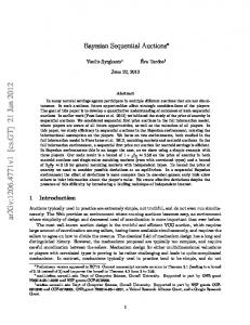
• Case-1: . In this case, target response appears in the channel only. and • Case-2: . In this case, varies at different frequencies. Under the Laplacian noise case, the number of antennas is limited to due to computational constraints. In this case, for each observation, we use substitute the Laplacian density for in (23) and evaluate the integral. This numerically constructed likelihood is used in sequential (numerical) evaluation of posterior density (21) and the posterior mean (24). Next, we examine the performance of the proposed waveform design and the sequential estimator using the metrics described below. A. SNR Gain In Fig. 1(a), the solid lines in this figure indicate the analytically evaluated SNR gain and the markers indicate the asymptotic values from the numerical simulations. For both the adaptive methods MCE and MCMI, the asymptotic SNR gain is very close to the theoretical SNR gain ( dB) at for Case-1. For the non-adaptive method EPA the computed SNR gain exactly matches with the theoretical value (0 dB). Fig. 1(b) illustrates the SNR gain as a function of number of antennas in the array . The SNR gain computed correin Case-2 for different sponds to the channel values of . These numerical results (markers) agree well with both the theoretical SNR gain (solid lines) evaluated using (55) and the bounds for SNR gain in (56). B. Asymptotic Estimation Error Bound and Convergence An estimator is considered asymptotically efficient if its error variance asymptotically reaches the BCRB [28], [48]. The average variance defined below is a measure of accuracy of the estimator [28]. (67) Next, we examine the estimation performance under Gaussian noise model (see Fig. 2) and Laplacian noise model (see Fig. 3), respectively, for simulation Case-2. Fig. 2(a) presents the simulation based average asymptotic BCRB (the line with markers) and its theoretical value (the solid line) versus the variance in a logarithmic scale. It can be seen that the posterior variance reaches the asymptotic BCRB as the number of iterations becomes large. Hence, both MCE and EPA are asymptotically efficient. The asymptotic convergence of the variance toward very low values illustrates the accuracy of the estimator. For the methods MCE and MCMI, Fig. 2(b) shows that the value under the stopping criterion in (25) reaches the tolerance level of (indicated by the red cycles. These results show that the sequenline) after at tial estimator MCE converges to the true parameter values faster than the non-adaptive algorithm EPA and the adaptive method MCMI. Similar performance is also observed under a non-Gaussian noise model. Fig. 3 depicts the asymptotic Bayesian CRB and the convergence speed for the MCE, MCMI and the non-adaptive EPA method under the Laplacian noise model. It is clear that, in the presence of Laplacian noise, the MCE method shows a smaller error bound (see Fig. 3(a)) and a faster convergence

Fig. 1. (a) SNR gain in dB vs. parameter in Case-1. (b) SNR gain in dB vs. for the frequency channel in Case-2. number of antennas

(see Fig. 3(b)) than the benchmark approaches MCMI and EPA methods. C. Conditional Entropy and Mutual Information Gain We examine the relationship between the error variance, the BCRB bound, and the conditional entropy and mutual information gain by numerical means. Fig. 4(a) illustrates the average entropy for the three channels in the Case-2 discussed in Section V.A. In this plot, the initial value 6.6 corresponds to the maximum possible uncertainty regarding and is given by . Here is the total number of possible values for randomly samprior to any measurements. Hence, pled from the interval . The final value is calculated from the conditional entropy using the posterior pdf when the stopping criterion is met. Next, comparing the entropy plot in Fig. 4(a) with the logarithm plot of average variance in Fig. 2(a), we observe that there is a linear relationship between the entropy and

TURLAPATY AND JIN: BAYESIAN SEQUENTIAL PARAMETER ESTIMATION

Fig. 2. Performance under Gaussian noise. (a) Asymptotic BCRB vs. iterations (in cycles). (b) Adaptive algorithms MCE and MCMI result in accelerated convergence towards their true estimates than the non-adaptive algorithm EPA.

the quantity . This observation is confirmed by a simple linear regression analysis, which yields (68) By comparing the (68) with (44) we see that for a Gaussian density the scaling factor is and the constant . Here we have which means that the pdf of is non-Gaussian because of the non-linear reand the measurements. The average statistics lation between across the frequency channels for different methods are presented in the Table II. In the regression analysis, we observe that the relation (68) is strong as becomes larger, i.e., as the estimation process reaches convergence. Note that in regression, the coefficient of determination is a statistical measure of how well the regression line approximates the real data points. An of 1.0 indicates that the regression line perfectly fits the data. Basically, this relation supports the hypothesis that minimization of entropy minimizes the posterior error

983

Fig. 3. Performance under Laplacian noise. (a) Asymptotic BCRB vs. iterations (in cycles). (b) Adaptive algorithms MCE results in accelerated convergence towards their true estimates than the EPA and MCMI.

variance. The mutual information gain (MIG) defined in (58) between MCE and EPA is shown as , which can be interpreted as the improvement of the asymptotic Bayesian Cramer-Rao bound between these two methods. Note that the relation in (68) can be extended to asymptotic BCRB as (i.e., when becomes large) (69) For the non-adaptive case the corresponding relation is (70) Hence, by simple algebraic manipulations, the improvement factor in asymptotic BCRB due to waveform adaptation is (71) where the exponent term . By plugging the regression coefficients in Table II (i.e.,

984

IEEE TRANSACTIONS ON SIGNAL PROCESSING, VOL. 63, NO. 4, FEBRUARY 15, 2015

Fig. 5. Asymptotic error variance vs. number of antennas over the three frequencies under Gaussian noise for Case-2.

averaged

D. Influence of the Size of Antenna Array on Error Variance Fig. 5 depicts the improvement in asymptotic error variance defined in (67) as the number of antennas (here we assume ) increases for the three methods under Case-2. The plots are averaged over the frequency channels. The vertical axis is in logarithmic scale. The plots show that, for a large array size (in this case ), the adaptive waveform methods MCE and MCMI show increasingly large improvement of asymptotic error variance over the non-adaptive method EPA. The main reasons for this improvement are spatial diversity due to the use of antenna arrays and adaptive power allocation of the waveform. As the number of antennas increase, the size of the target covariance matrix also increases, which give rises to higher degrees of freedom for waveform’s spatial diversity. E. Computational Complexity Fig. 4. Averaged conditional entropy vs. iterations averaged over the frequencies for Case-2. (a) Under Gaussian noise model. (b) Under Laplacian noise model. TABLE II REGRESSION ANALYSIS OF CONDITIONAL ENTROPY AND

) and the reading in Fig. 4(a) into (71), we obtain the improvement in asymptotic BCRB for MCE relative to EPA as . This value matches with the reading at final iteration between the MCE plot and the EPA plot shown in Fig. 2(a). Similarly, Fig. 4(b) and Table II show that, conditional entropy of MCE is smaller than that of MCMI and EPA in the presence of Laplacian noise. Comparing Fig. 4(b) and (a), we show that MCMI is sensitive to the noise models.

We use the big-O notation, [49], to represent the computational complexity of the three algorithms: the non-adaptive method EPA and the adaptive methods MCE and MCMI under Gaussian noise and Laplacian noise, respectively, which are summarized in Table III. Under the Gaussian noise model, we let denote the complexity for EPA, which consists of the following computational operations: (1) matrix vector multiplication , where is the number of parallel processes available in the computer platform; (2) Bayesian transformation with complexity , where is the number of samples; (3) estimation of the mean and variance with complexity , (4) computation of ABCR bound ; and (5) computation of conditional entropy . The complexity of the adaptive methods is combined computation of the EPA and the additional complexity of computing the waveform at each cycle, i.e., . denote the complexity for waveform design where for MCE and MCMI, respectively. For MCE, the waveform computation involves the computation of the objective function and its Hessian matrix numerically. The two steps are repeated times before convergence is reached, while each repetition involves computing the entropy using numerical integration . For MCMI, the computation of

TURLAPATY AND JIN: BAYESIAN SEQUENTIAL PARAMETER ESTIMATION

TABLE III COMPUTATIONAL COMPLEXITY PER TRANSMISSION CYCLE

involves three steps: (1) eigen decomposition of the covariance matrix ; (2) water filling algorithm ; and (3) matrix multiplication . Under the Laplacian noise model, we let denote the complexity for EPA. is the number of values on the real line in one dimension of the vector of dimension . In each dimension, the numerical integration involves evaluation of the integrand function and weighted summation in that dimension which has complexity . Later, we repeat this process in dimensions, the complexity is . Next for both the adaptive methods we have the additional complexity of the waveform design that involves the computation of the objective function and its Hessian matrix numerically. The two steps are repeated times before convergence is reached. For MCE, each repetition involves computing the likelihood function and the conditional entropy using nu. For merical integration with complexity MCMI, the two steps are (i) the computation of the likelihood function and (ii) the conditional entropy of given , and . each step has complexity We implement the three algorithms in Matlab on a Dell Optiplex 64-bit desktop computer. Under Gaussian noise model, the processing times of one transmission cycle for the three methods are s, s and s. Under Laplacian noise model, the processing times of one transmission cycle for the three methods are s, s and s. Here each of the channels are processed one at a time. The results show that the complexity of MCMI is comparable to that of EPA (because is much larger ) and is less than that of MCE. F. Comparison of MCE and MCMI Under Gaussian and Laplacian Noise The two adaptive methods MCE and MCMI are based on and two different mutual information quantities , respectively. The method MCE yields the optimal solution in that it minimizes directly the posterior entropy of the parameter. However, the MCE does not have an analytical solution and is computed using numerical means. The method MCMI maximizes the mutual information indirectly with the parameter through the , thus a suboptimal method. The channel measurement performance gain in terms of Bayesian CRB, convergence speed of sequential estimator of MCE over MCMI is clearly demonstrated in Figs. 2, 3 and 4. Moreover, results in Fig. 4(b) and (a) show that MCMI is sensitive to the noise models. Nevertheless, the advantage of MCMI is that, under the Gaussian assumptions (i.e., Gaussian channel and Gaussian noise), it has

985

an analytical solution and thus with less computational complexity. Moreover, its performance is similar to MCE because, under the Gaussian assumption, the mutual has a linear relation with the mutual information . This can be verified by comparing the entropy given in Fig. 4(a) with the conditional entropy derived from (36) given by . For instance, by linear regression, we determine that the linear relation can be presented as , where and for with . Finally, it is not difficult to show that under a special case when there exists a linear relationship between the target response and the parameter of interest , the two methods MCE and MCMI are the same. VI. CONCLUSION We have developed an integrated approach of adaptive waveform design and Bayesian sequential estimation in the framework of cognitive radar. The adaptive method transmits new waveform and updates the posterior probability estimate recursively in response to the new measurements and channel condition. The main finding is that with the use of adaptive waveform the sequential Bayesian estimator achieves improved accuracy (i.e., smaller error variance), faster convergence and lower conditional entropy (i.e., less uncertainty). The improvement results from the adaptation of the waveform structure and spatial diversity of the antenna array. The theoretical analysis of the signal-to-noise ratio gain, the conditional entropy and the asymptotic Bayesian Cramer Rao bound of the estimator show the advantage of the proposed adaptive Bayesian estimator compared with the conventional non-adaptive Bayesian sequential estimation method. APPENDIX A WAVEFORM DESIGN BASED ON MUTUAL INFORMATION Consider the optimization problem given in (47), the objective function can re-written using the eigen decomposition of the covariance matrix based on the latest estimate of , which yields (72) Next we let (73) then (72) becomes By using the matrix identity and letting

. , [36], (74)

we obtain (75) is a diagonal matrix, Since it is straightforward to see that (75) is maximized when the matrix is also diagonal given in (49). Thus the optimization problem in (47) becomes

(76)

986

IEEE TRANSACTIONS ON SIGNAL PROCESSING, VOL. 63, NO. 4, FEBRUARY 15, 2015

Using a lagrange multiplier the optimization can be re-written as

at least two entries the rest entries to the constraint that

and for

. Note that

(84) (85)

(77) Differentiating with respect to

yields (78)

Hence, the solution is , which implies that the energy allocation term can be determined by a water-filling algorithm ([4], [12], [18]) as (79) where is the water level. Considering the energy constraint in (76), (79) becomes

Equations (84)–(85) show that the minimum value of the inner is reached if the entries of the vector are all product equal. Next, we let the diagonal eigen-matrix of the covaribe sorted in a descending order, i.e., ance matrix (86) . We also consider where a general water-filling type solution with the condition in (86) and the constraint , where (87) Inserting (87) in (55) yields

(80) Hence, using (74) and (73), we obtain , which yields (48), where is obtained by the singular value decomposition of , where is the singular value matrix and are the right singular vector matrix. Based on [12], must comprise of orthogonal vectors.

. For due . Then

(88) Using Lemma 2.1, it is straightforward to show that when , the lower bound is (89) Similarly, the upper bound is obtained as

APPENDIX B BOUNDS ON SNR GAIN

(90)

Lemma 2.1: Let and are two vectors. Assuming that entries of the given vector is sorted in a descending order, i.e., and the vector is subject to the constraint and . is a constant. The inner product reaches (i) the maximum value if the entries of are and (ii) the minimum value if . Proof: Part (i). Suppose that the entries of are not in a descending order. Then there must be entries and for which but . This is essentially a statement that is not sorted. Next, we sort this vector by swapping these two entries, which yields a new vector . The vector is the same as vector except that and . Note that (81) (82) (83) Equations (81)–(83) show that the maximum value of the inner product is reached if the entries of the vector are sorted in a descending order. Part (ii). Next, we use proofs by contradiction to show that the minimum value is reached if . Suppose that the entries of the vector is all equal, i.e., , and that a new vector will result in a smaller inner product with

REFERENCES [1] S. Haykin, “Cognitive radar: A way of the future,” IEEE Signal Process. Mag., vol. 23, no. 1, pp. 30–40, Jan. 2006. [2] G. T. Capraro, A. Farina, H. Griffiths, and M. C. Wicks, “Knowledgebased radar signal and data processing: A tutorial review,” IEEE Signal Process. Mag., vol. 23, no. 1, pp. 18–29, Jan. 2006. [3] N. A. Goodman, P. R. Venkata, and M. A. Neifeld, “Adaptive waveform design and sequential hypothesis testing for target recognition with active sensors,” IEEE J. Sel. Topics Signal Process., vol. 1, no. 1, pp. 105–113, Jun. 2007. [4] R. A. Romero and N. A. Goodman, “Waveform design in signal-dependent interference and application to target recognition with multiple transmissions,” IET Radar, Sonar Navig., vol. 3, no. 4, pp. 328–340, 2009. [5] P. Chavali and A. Nehorai, “Scheduling and power allocation in a cognitive radar network for multiple-target tracking,” IEEE Trans. Signal Process., vol. 60, no. 2, pp. 715–729, Feb. 2012. [6] U. Gunturkun, “Toward the development of radar scene analyzer for cognitive radar,” IEEE J. Ocean. Eng., vol. 35, no. 2, pp. 303–313, Apr. 2010. [7] P. Dayan, G. E. Hinton, and R. M. Neal, “The Helmholtz machine,” Neural Comput., vol. 7, pp. 889–904, 1995. [8] T. S. Lee and D. Mumford, “Hierarchical Bayesian inference in the visual cortex,” J. Opt. Soc. Amer. A. Opt., Image Sci. Vis., vol. 20, no. 7, pp. 1434–1448, Jul. 2003. [9] D. Kersten, R. Mamassian, and A. Yuille, “Object perception as Bayesian inference,” Ann. Rev. Psychol., vol. 55, pp. 271–304, 2004. [10] D. C. Knill and A. Pouget, “The Bayesian brain: The role of uncertainty in neural coding and computation,” Trends in Neurosci., vol. 27, pp. 712–719, 2004. [11] J. V. Candy, Bayesian Signal Processing. Hoboken, NJ, USA: WileyIEEE, 2009.

TURLAPATY AND JIN: BAYESIAN SEQUENTIAL PARAMETER ESTIMATION

[12] Y. Yang and R. S. Blum, “MIMO radar waveform design based on mutual information and minimum mean-square error estimation,” IEEE Trans. Aerosp. Electron. Syst., vol. 43, no. 1, pp. 330–343, Jan. 2007. [13] M. Alvo, “Bayesian sequential estimation,” Ann. Statist., vol. 5, no. 5, pp. 955–968, Sep. 1977. [14] K. G. Jamieson, M. R. Gupta, and D. W. Krout, “Sequential Bayesian estimation of the probability of detection for tracking,” in Proc. IEEE 12th Int. Conf. Inf. Fusion, Seattle, WA, USA, 2009, vol. 12, pp. 641–648. [15] D. S. Lee and N. K. K. Chia, “A particle algorithm for sequential Bayesian parameter estimation and model selection,” IEEE Trans. Signal Process., vol. 50, no. 2, pp. 326–336, Feb. 2002. [16] M. West, “Robust sequential approximate Bayesian estimation,” J. R. Statist. Soc. B, vol. 43, no. 2, pp. 157–166, Jul. 1981. [17] M. N. Desai and R. S. Mangoubi, “Robust subspace learning and detection in Laplacian noise and interference,” IEEE Trans. Signal Process., vol. 55, no. 7, pp. 3585–3595, Jul. 2007. [18] M. R. Bell, “Information theory and radar waveform design,” IEEE Trans. Inf. Theory, vol. 39, no. 5, pp. 1578–1597, Sep. 1993. [19] Y. Yang, R. S. Blum, Z. He, and D. R. Fuhrmann, “MIMO radar waveform design via alternating projection,” IEEE Trans. Signal Process., vol. 58, no. 3, pp. 1440–1445, Mar. 2010. [20] Y. Jin, J. M. F. Moura, and N. O’Donoughue, “Time reversal transmission in multi-input multi-output radar,” IEEE J. Sel. Topics Signal Process., vol. 4, no. 1, pp. 210–225, Feb. 2010. [21] Y. Jin and J. M. F. Moura, “Time reversal detection using antenna arrays,” IEEE Trans. Signal Process., vol. 57, no. 4, pp. 1396–1414, Apr. 2009. [22] Y. Jin, “Cognitive multi-channel radar detection using Bayesian inference,” in Proc. IEEE Sens. Array and Multi-Channel Signal Process. Workshop (SAM), Hoboken, NJ, USA, 2012, pp. 417–420. [23] B. Friedlander, “Adaptive waveform design for a multi-antenna radar system,” in Proc. IEEE Asilomar Conf. Siganls, Syst. Comput., Pacific Grove, CA, USA, 2006, pp. 735–739. [24] Y. Jin and B. Friedlander, “Adaptive processing of distributed sources using sensor arrays,” IEEE Trans. Signal Process., vol. 52, no. 6, pp. 1537–1548, Jun. 2004. [25] R. L. Mitchell, “Models of extended targets and their coherent radar images,” Proc. IEEE, vol. 62, no. 6, pp. 754–758, Jun. 1974. [26] A. Isbimaru, Wave Propagation and Scattering in Random Media. Piscataway, NJ, USA: Wiley-IEEE Press, Feb. 1999. [27] B. Porat, A Course in Digital Signal Processing. New York, NY, USA: Wiley, Oct. 1996. [28] S. M. Kay, Fundamentals of Statistical Signal Processing: Estimation Theory. Englewood Cliffs, NJ, USA: Prentice-Hall, 1993. [29] A. Papoulis, Probability, Random Variables and Stochastic Processes, 2nd ed. New York, NY, USA: McGraw-Hill, Mar. 1984. [30] U. Nickel, E. Chaumette, and P. Larzabal, “Estimation of extended targets using the generalized monopulse estimator: Extension to a mixed target model,” IEEE Trans. Aerosp. Electron. Syst., vol. 49, no. 3, pp. 2084–2096, Jul. 2013. [31] P. Swerling, “Radar probability of detection for some additional fluctuating target cases,” IEEE Trans. Aerosp. Electron. Syst., vol. 33, no. 2, pp. 698–709, Apr. 1997. [32] R. S. Raghavan, “A model for spatially correlated radar clutter,” IEEE Trans. Aerosp. Electron. Syst., vol. 27, no. 2, pp. 268–275, Mar. 1991. [33] V. A. Aalo, “Performance of maximal-ratio diversity systems in a correlated Nakagami-fading environment,” IEEE Trans. Commun., vol. 43, no. 8, pp. 2360–2369, Aug. 1995. [34] A. A. Monakov, “Observation of extended targets with antenna arrays,” IEEE Trans. Aerosp. Electron. Syst., vol. 36, no. 1, pp. 297–302, Jan. 2000. [35] J.-H. Chang, “Complex Laplacian probability density function for noisy speech enhancement,” IEICE Electron. Expr., vol. 4, no. 8, pp. 245–250, 2007. [36] G. H. Golub and C. F. Van Loan, Matrix Computations, 3rd ed. Baltimore, MD, USA: The Johns Hopkins Univ. Press, Oct. 1996. [37] D. Guo, S. Shamai, and S. Verdu, “Mutual information and minimum mean-square error in Gaussian channels,” IEEE Trans. Inf. Theory, vol. 51, no. 4, pp. 1261–1282, Apr. 2005. [38] Y. Wu and S. Verdu, “Functional properties of minimum mean-square error and mutual information,” IEEE Trans. Inf. Theory, vol. 58, no. 3, pp. 1289–1301, Mar. 2012. [39] F. Kanaya and K. Nakagawa, “On the practical implication of mutual information for statistical decisionmaking,” IEEE Trans. Inf. Theory, vol. 37, no. 4, pp. 1151–1156, Jul. 1991. [40] T. M. Cover and J. A. Thomas, Elements of Information Theory, 2nd ed. Hoboken, NJ, USA: Wiley-Interscience, Jul. 2006.

987

[41] P. E. Gill, W. Murray, and M. H. Wright, Practical Optimization. London, UK: Academic, 1982. [42] S.-P. Han, “A globally convergent method for nonlinear programming,” J. Optimiz. Theory Appl., vol. 22, no. 3, pp. 297–309, Jul. 1977. [43] D. J. Johnson and D. E. Dudgeon, Array Signal Processing: Concepts and Techniques. Upper Saddle River, NJ, USA: Prentice-Hall, Feb. 1993. [44] W. Yu and J. M. Cioffi, “Constant-power waterfilling: Performance bound and low-complexity implementation,” IEEE Trans. Commun., vol. 54, no. 1, pp. 23–28, Jan. 2006. [45] H. L. Van Trees, Detection, Estimation, and Modulation Theory, Part I. Hoboken, NJ, USA: Wiley-Interscience, Sep. 2001. [46] J. Dauwels, “Computing Bayesian Cramer-Rao bounds,” in Proc. Int. Symp. Inf. Theory, Sep. 2005, pp. 425–429. [47] L. Zuo, R. Niu, and R. K. Varshney, “Conditional posterior Cramer Rao lower bounds for nonlinear sequential Bayesian estimation,” IEEE Trans. Signal Process., vol. 59, no. 1, pp. 1–14, Jan. 2011. [48] P. Stoica and A. Nehorai, “MUSIC, maximum likelihood, and Cramer-Rao bound,” IEEE Trans. Acoust., Speech Signal Process., vol. 37, no. 5, pp. 720–741, May 1989. [49] T. H. Cormen, C. E. Leiserson, R. L. Rivest, and C. Stein, Introduction to Algorithms, 3rd ed. Cambridge, MA, USA: The MIT Press, Jul. 2009.

Anish Turlapaty (S’08) received the B.Tech. degree in electronics and communication engineering from Nagarjuna University, India, in 2002, the M.Sc.degree in engineering degree in radio astronomy and space sciences from the Chalmers University, Sweden, in 2006, and the Ph.D. degree in electrical engineering from the Mississippi State University, Mississippi State, in 2010. From July 2010 to January 2012, he was at Mississippi State as a postdoctoral associate working on pattern recognition and digital signal processing based methods for detection of subsurface radioactive waste using electromagnetic induction spectroscopy. He is a Postdoctoral Research Associate in the Department of Engineering and Aviation Sciences, University of Maryland Eastern Shore. He is currently working on digital signal processing for cognitive radar systems. Dr. Turlapaty received Graduate Student of the Year Awards for outstanding research from both the Mississippi State University Centers and Institutes and the Geo-systems Research Institute at Mississippi State University in 2010. He has published 8 peer-reviewed journal papers and presented 12 papers and posters at international conferences and symposia. He is also an active reviewer for many international journals related to signal processing.

Yuanwei Jin (S’99–M’04–SM’08) received the Ph.D. degree in electrical and computer engineering from the University of California at Davis in 2003. From 2003 to 2004, he was a Visiting Researcher with the University of California at Santa Cruz. From 2004 to 2008, he was a Postdoctoral Research Fellow, then Project Scientist, with the Department of Electrical and Computer Engineering, Carnegie Mellon University, Pittsburgh, PA. From August 2008 to July 2012, he was an Assistant Professor with the Department of Engineering and Aviation Sciences at the University of Maryland Eastern Shore. Since August 2012, he has been an Associate Professor. From August 2010 to June 2012, he was the Interim Department Chair. He is an Associate Professor of Electrical Engineering with the Department of Engineering and Aviation Sciences of the University of Maryland Eastern Shore, Princess Anne, MD. His research interests are in the general area of signal processing, sensor array processing, and computational inverse problems, with applications in radar/sonar, biomedical imaging, structural health monitoring, and nonintrusive load monitoring for energy management. He holds two U.S. patents. Dr. Jin received a 2010 Air Force Summer Faculty Fellowship award. He was a recipient of an Earle C. Anthony Fellowship from the University of California at Davis. He is affiliated with several IEEE societies, Sigma Xi, SPIE, and the American Society for Engineering Education (ASEE).