cheap devices with many integrated sensors and wireless communication .... laptops. Each test consists in 50 sequences of 100 packets for each packet size sent at maximum power (0 ...... to work on different delay functions to deal with.
Month 200X, Vol.21, No.X, pp.XX–XX
J. Comput. Sci. & Technol.
Beacon-less Geographic Routing in Real Wireless Sensor Networks Juan A. Sanchez1 , Rafael Marin-Perez1 , and Pedro M. Ruiz1 1 Dept.
Information and Comms. Eng., University of Murcia, Spain
E-mail: {jlaguna, rafael81, pedrom}@dif.um.es Received MONTH DATE, YEAR. Abstract
Geographic Routing (GR) algorithms, require nodes to periodically transmit HELLO
messages to allow neighbors know their positions (beaconing mechanism). Beacon-less routing algorithms have recently been proposed to reduce the control overhead due to these messages. However, existing beacon-less algorithms have not considered realistic physical layers. Therefore, those algorithms cannot work properly in realistic scenarios. In this paper we present a new beacon-less routing protocol called BOSS. Its design is based on the conclusions of our open-field experiments using Tmote-sky sensors. BOSS is adapted to error-prone networks and incorporates a new mechanism to reduce collisions and duplicate messages produced during the selection of the next forwarder node. We compare BOSS with Beacon-Less Routing (BLR) and Contention-Based Forwarding (CBF) algorithms through extensive simulations. The results show that our scheme is able to achieve almost perfect packet delivery ratio (like BLR) while having a low bandwidth consumption (even lower than CBF). Additionally, we carried out an empirical evaluation in a real testbed that shows the correctness of our simulation results. Keywords
1
geographic routing, beacon-less forwarding, performance evaluation, real deployment
Introduction
cheap devices with many integrated sensors and wireless communication interfaces.
In the last few years, Wireless Sensor
Nodes
use
their
wireless
radio
to
Networks (WSN) have become a hot topic not
communicate the information acquired with
only for researchers but also for the industry.
their sensors. When the destination is out of
A WSN consists of a big set of lightweight and
the radio range of the source node, other nodes
∗
This work is supported by Spanish MEC under Grant No TIN2005-07705-C02-02 and the “Ramon y Cajal”
work programme.
2
J. Comput. Sci. & Technol., Month 200X, Vol.21, No.X
are used as relay stations.
selects the next forwarder among its neighbors
Geographic Routing (GR) is one of the
after determine their positions.
schemes which has gained most momentum in
These algorithms are reported to work fine
recent years. In GR each node needs to know
according to the results of several simulations.
the position of its neighbors.
Thus, nodes
Nevertheless, most of the beacon-less protocols
periodically send short HELLO messages called
reported in the literature assume a perfect
beacons including the identifier and position of
wireless channel and do not consider the
the sender. These packets are not forwarded,
problems of losses and interferences created by
therefore only one hop neighbors can receive
the transmission of messages during the next
them.
forwarder selection process.
As it has been
although GR in general is
shown recently ([5,6]), there are huge differences
highly desirable, the beaconing mechanism
between a real link and a simulated one using
has some drawbacks.
the well known unit disk model generally
However,
For example, beacons
can interfere with regular data transmission
accepted in the literature.
and their bandwidth and battery power
realistic link layer has big implications on
consumption cannot be underestimated.
the performance and validity of the proposed
In
particular in those sensors not taking part in any routing process,
the energy and
Considering a
algorithms. In
this
paper,
we
propose
BOSS,
bandwidth consumption represents a total
the Beacon-less On Demand Strategy for
waste of resources. To overcome such issues
Geographic
Routing
several beacon-less routing protocols have been
Networks.
Its design takes into account
proposed for WSNs. The most representative
the losses and collisions typical of radio
examples are: IGF [1], GeRaF [2], CBF [3], and
communications.
BLR [4].
a practical study to determine the impact of
in
Wireless
Sensor
Concretely, we have made
Beacon-less routing protocols do not require
the packet size on the Packet Reception Ratio
any proactive transmission of control messages
(PRR). As our experiments confirm, bigger
which saves network resources.
In these
packets are more likely to be lost. Thus, unlike
algorithms, the next forwarder is reactively
previous schemes, BOSS starts sending out the
selected. There are two main approaches for
data packet itself rather than a control message.
selecting the next forwarder node. In the first
By doing that, only the neighbors able to receive
one the neighbors collaboratively decide which
the data packet contend for becoming the next
one must be the next forwarder. In the second
forwarder.
one the node currently holding the message
BOSS uses also a passive ACK scheme
Juan A. Sanchez et al.:BOSS: Beaconless On-demand Strategy for Geographic Routing
to reduce the control overhead.
3
We also
it is possible to reach a node where no neighbor
introduce the Discrete Dynamic Forwarding
closer to the destination exists. In those cases,
Delay (DDFD) a new timer-based contention
a recovery strategy must be used to surround
scheme to achieve a reduction of the collisions
the void area reached. This is called perimeter
of the answers during the selection phase.
routing and it is based in the application of
The remainder of this paper is organized as follows.
Section 2, gives an overview of
existing geographic routing protocols.
The
routing algorithm BOSS is described section 3.
Section 3.1,
in
discusses some
variations and optimizations of BOSS. Then
the right-hand rule [9] over a planarized vision of the underlying graph.
The combination
of a greedy approach and a recovery strategy is widely used in the literature.
The most
well-known algorithm doing that is Greedy Face Greedy Routing [10].
Section 4 evaluates the performance of BOSS
GR algorithms usually employ a beaconing
through simulations and compares it to existing
mechanism to know neighbors positions. Some
solutions in the literature. Section 5 presents
of the beacons may be useless if data packets
the results of our performance evaluation in a
are not routed through some of the nodes.
real wireless sensor network testbed. Finally,
Moreover,
section 6 concludes this paper.
limitations that these algorithms have when
recent studies have shown the
mobility is taken into account[11,12]. 2
To avoid these periodic transmissions,
Related work
beacon-less protocols have been proposed in the literature. The general idea of beacon-less have
is to reactively discover the information about
become very popular in the field of WSNs
neighbors’s positions just when routing data
because of their localized operation, reduced
packets.
Geographic
Routing
algorithms
computation and storage requirements and,
The Implicit Geographic Forwarding [1]
above all, because of their scalability with the
(IGF) is a state-free routing protocol.
number of nodes [7,8].
is a modification of the 802.11 DCF MAC
The idea of geographic algorithms is to forward the packet in the direction of the
IGF
protocol adding to the RTS/CTS handshaking a DATA/ACK interchange.
If the density of nodes is high
Authors introduce the idea of delaying the
enough, at each step the packet can be moved
transmission of the CTS to avoid collisions.
to a node closer to the destination than the
They define a function for computing that
previous one. This is called greedy routing, but
delay according to the distance towards the
destination.
4
J. Comput. Sci. & Technol., Month 200X, Vol.21, No.X
Thus, farther
Additionally, a recovery strategy is defined.
neighbors answer before the nodes placed closer
The forwarder node rebroadcasts the packet
to the current one.
if it does not hear any retransmission during
destination of each neighbor.
A similar scheme is also used in the
a predefined time interval.
In this case,
Geographic Random Forwarding [2] (GeRAF)
all the neighbors must answer with their
protocol. The main difference is that GeRAF
positions. The forwarding node then, is able
uses two different frequencies for the collision
to locally build the planar graph and using the
avoidance MAC scheme. More recently, a newer
recovery scheme of GFG [10] determine the next
paper from the same authors [13] presented
forwarding node in perimeter mode.
an extension of GeRAF. This variant called GeRaF-1R does collision resolution with a
The
Contention-Based
Forwarding
Candidate relays
algorithm [3] (CBF) mixes the centralized
schedule the forwarding of received messages
selection of the next forwarder based in a
by means of a probabilistic approach. Doing
RTS/CTS/DATA process with a delimited
so they are able to reschedule the operation
Forwarding Area whose goal is reducing the
avoiding the possible collisions.
duplicates in the same way as in BLR.
single radio frequency.
Lately, Heissenb¨ uttel et al. proposed a new algorithm called Beacon-Less Routing[4] (BLR)
The Blind Geographic Routing [14] (BGR)
which follows a different approach. In BLR,
protocol is very similar to BLR. The novelties
the selection of the next forwarder is totally
introduced are a different recovery process and
distributed.
a strategy to avoid the problem of simultaneous
That is, the current forwarder
just broadcasts the data packet and the closest
forwarding.
The results achieved are very
neighbor to the destination resends the packet
similar to the ones of BLR.
because its timer expires in the first place. The rest of neighbors hearing the transmission
Finally, Chawla et al.
[15] proposed a
cancel their timers. To avoid duplications due
new delay function to reduce the number of
to neighbors not hearing transmissions, the
neighbors replying in perimeter mode.
authors determine that only the nodes located
function assigns shorter delays to neighbors
in a specific area, denominated Forwarding
closer to the forwarding node.
Area, can participate in the process. This area
farther neighbors can cancel their responses
is relative to the forwarding node and can be
after hearing the perimeter response of other
of any shape provided that all nodes within the
neighbors, because they determine they are not
area can overhear each other.
part of the planar graph of the forwarding node.
This
Therefore,
Juan A. Sanchez et al.:BOSS: Beaconless On-demand Strategy for Geographic Routing
3
Beacon-less Routing with BOSS
5
of being received than smaller ones. If that is the case, discovering the neighborhood using one small control packet may cause to select
BOSS
uses
a
three
way
handshake
mechanism to select and forward messages in a similar way to the RTS/CTS scheme used in IEEE 802.11. Firstly the forwarding node broadcasts the data at maximum power to reach all its possible neighbors and waits for the first response of a neighbor. Then it confirms the selection with a final control packet. The key aspect of BOSS is the way of discovering the neighborhood. To do that, instead of using a control packet we use the data packet. Data messages are bigger than control messages, so that, they are more likely to be lost. Thus, the idea behind BOSS is to use the data packet being routed to discover the neighbors. In that way, neighbors not able to receive a packet of that size due to wireless errors will not take part in the selection process. To confirm the importance of the packet size in the percentage of packets received and, therefore, support the goodness of our idea, we have made some experiments whose results are shown in the next section.
a neighbor which may not be able to receive the bigger data packet. Our goal is to validate such assumption. Therefore, we run a set of real experiments in order to obtain the relation between Packet Size and the Packet Reception Ratio. We use are the new Tmote-sky [16] sensors based on the CC2420 radio chip from Chipcon [17].
The main elements integrated on the
Tmote-sky, are the following:
a MSP430
microcontroller (with 10kB RAM memory and 48kB Flash memory), a CC2420 radio chip (based in standard IEEE 802.15.4), an omnidirectional antenna (that provides a radio range of up to 50 meters indoor and 125 meters outdoor) and optionally, sensors of humidity, temperature, and light to monitor the environment. The measurements have been obtained in an outdoor area of 100x100 meters. We use two sensors (source and receiver) placed at 0,5m above the ground and connected via USB to laptops.
Each test consists in 50 sequences
of 100 packets for each packet size sent at 3.1
Analysis of the CC2420 Radio
maximum power (0 decibel) by the source node. The receiver reports to its connected laptop the
The BOSS protocol is based on the
following measured parameters:
assumption that the size of the packets has a direct relationship with the probability of error. Concretely, bigger packets have less probability
• RSSI.
The
Radio
Signal
Strength
Indicator is a 8-bit value given by CC2420
6
J. Comput. Sci. & Technol., Month 200X, Vol.21, No.X 120 10 bytes 25 bytes 40 bytes 55 bytes 70 bytes 85 bytes 100 bytes 115 bytes
Packet Reception Ratio (PRR)
100
80
60
40
20
0 10
20
30
40 41 42 43 44 45 46 47 48 49 50 51 60 Distance (meters)
80
100
120
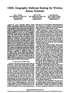
Figure 1: Percentage of messages successfully transmitted at varying the distance for different packet sizes using the CC2420 radio interface.
chip that indicates the received signal
in the range between 44 and 51 meters have
strength in decibel.
greater variability, the resolution in that range
• LQI. The Link Quality Indicator can be viewed as the chip error rate.
It is
calculated over 8 bits following the start frame delimiter (SFD). The LQI values are usually between 110 and 50, and correspond to maximum and minimum quality frames respectively.
is greater. Fig. 1 summarizes the results of our experiments. It shows the value of the PRR at varying the distance. Each curve represents the data obtained with each packet size tested. The packet size is the sum of the payload and the headers of the MAC and link layer. The first conclusion that we can extract
• PS. The Packet Size is the sum of the payload size and header size of the received packet.
is that, as we anticipated, the greater the packet size, the lower the PRR. The second conclusion is that there is no direct relation
The Packet Reception Ratio (PRR) is
between the distance and the PRR. As it can
computed in the laptop and it is defined as the
be seen, the results at some distances such
ratio between the number of packets received
as 48m and 46m, are better than at some
and the total number of packets sent.
other shortest distances, respectively 47m and
We have performed tests using 8 different
45m. This coincides with some other empirical
payload sizes (10, 25, 40, 55, 70, 85, 100 and 115
results[18][19][20] that show the irregularities of
bytes) and varying the distance between source
wireless communications in WSNs.
and receiver (from 5m to 120m). As the results
Moreover, as it can be seen, sensors placed
Juan A. Sanchez et al.:BOSS: Beaconless On-demand Strategy for Geographic Routing
7
farther than 51m are not able to communicate
node and the final destination’s position. Each
directly.
Although the maximum theoretical
neighbor receiving the message stores it and
range is 125m, placing the sensors near the floor
determines the relative area in which it is
causes too much reflections. In some other tests
located (PPA or NPA). Finally, instead of
done with sensors placed at 2m above the floor,
answering immediately, the node starts a
the range grows up to 150m.
timer whose value depends on its position. When the timer finishes the neighbor broadcast
3.2
Forwarding in BOSS
BOSS uses four different types of messages: DATA, RESPONSE, SELECTION and ACK.
a RESPONSE message.
The RESPONSE
message contains the neighbor position and its identifier.
In addition, given the forwarding node (i.e.
Each neighbor in the PPA receiving a
the node currently holding the message)
RESPONSE message from another neighbor in
we define two relative areas around it.
the same area, cancels its timer and deletes
The Positive Progress Area (PPA) and the
the stored message. The RESPONSE messages
Negative Progress Area (NPA). PPA comprises
from NPA neighbors do not cancel any timer.
each node whose position is closest to the
Notice that it is possible that some neighbors
destination than the forwarding node while the
do not receive this message because of their
NPA comprises the rest of neighbors of the
positions.
forwarding node. That is, those not providing
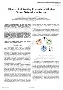
situation, in which, neighbors n1 and n3 cannot
progress towards the destination. Additionally,
hear the RESPONSE messages from each other.
the DATA, RESPONSE and SELECTION
The forwarding node stops its timer if a
messages include a bit in their headers to
RESPONSE message from a PPA neighbor is
indicate the routing mode currently being used
received.
(Greedy or Perimeter). This bit is called the
message. This message contains the identifier
Routing Mode bit (RM). The RM bit is set
of the neighbor selected by the forwarding node
to G mode by default. We now describe the
to become the next forwarding node.
detailed operation of the protocol, firstly in the
neighbor is the one whose RESPONSE message
greedy and then in perimeter mode.
arrived in the first place to the forwarding
Fig. 2 shows an example of this
It then broadcasts a SELECTION
That
In greedy mode, the forwarding node sends
node. More than one RESPONSE message from
a broadcast with a DATA message and waits
PPA neighbors might arrive to the forwarding
for responses for a predefined maximum time of
node but only the first one is used.
T Max seconds. The DATA message contains the
neighbor receiving the SELECTION message
original message, the position of the forwarding
will immediately cancel its timer and delete the
Each
8
J. Comput. Sci. & Technol., Month 200X, Vol.21, No.X
n1 n5
c n4
n2
r
d
n3
Area Progreso Positiva Area Progreso Negativa
Figure 2: Node c currently holding the message toward d and its neighbors. Nodes n1 , n2 and n3 are in the Positive Progress Area. Nodes n4 and n5 are in the Negative Progress Area. Nodes n1 and n3 cannot hear each other replies.
stored message except for the one selected by
in BOSS, the RESPONSE messages from
the forwarding node. The selected node knows
neighbors in the NPA do not cancel any timer.
it is the new forwarding node by examining the
Thus, when the forwarding node does not have
header of the SELECTION message. Finally,
any neighbor providing advance towards the
the new forwarding node starts again the
destination, all the RESPONSE messages from
protocol by broadcasting a new DATA message.
the other neighbors (those in the NPA area) are
Some nodes may not have any neighbors
received and stored. When the timer expires,
providing advance toward the destination. In
the forwarding node can thus build the planar
that case, a so-called void area, is found
graph using all the information gathered and
and the routing process cannot continue in
then selects the next forwarding node using the
greedy mode. In Geographic Routing protocols
desired recovery mechanism, in our case we use
there exist different strategies to surround these
the one proposed in GFG [10].
void areas but, usually, it is necessary to
In the case of perimeter routing the
know the position of the neighbors in order
SELECTION message must include some extra
to locally build a planar graph to determine
information. Concretely the identifier of the
the next perimeter forwarder.
The most
forwarding node, its position, identifier of the
common algorithms to do that are the Relative
next hop selected and the current perimeter
Neighbor Graph [21] (RNG) and Gabriel Graph
information defined by GFG which consists
[22] (GG). As we have already commented,
of: the position of the node where perimeter
Juan A. Sanchez et al.:BOSS: Beaconless On-demand Strategy for Geographic Routing
9
routing started (Lp ), the first edge (E 0 )
the implementation phase. As we have already
traversed on current face, and the (Lf ) point,
commented, the neighbors receiving a DATA
that is the cross point between the Lp D line
message store it and then wait for a timer
and the current face, being D the position of
to answer.
the destination node. Additionally, the RM bit
that data packet be stored. Obviously, if the
must be set to P indicating perimeter routing.
node receives a RESPONSE message, the data
The question is how long must
in
packet can be deleted. The same occurs after
perimeter routing, the behavior of neighbors is
receiving a SELECTION message directed to
slightly different. To begin with, the forwarding
another neighbor.
node must include in the DATA message the
with error-prone networks, both messages might
Lp point.
be lost.
When
messages
are
being
routed
A neighbor receiving the DATA
But, as we are dealing
In that case, the node will send
message must check if it is placed closer to the
its own RESPONSE message when its timer
destination than the Lp point. If that is the
expires.
case, it resumes to greedy mode. Thus, the
late response must ignore it, but the neighbor
RM bit of the RESPONSE message is set to G.
is waiting for a SELECTION message to select
Only in those cases, the RESPONSE message
it as next forwarder. This message will never
will be sent but, after the timer expires as in
arrive.
greedy routing. The forwarding node may stop
deleted after a maximum time.
its timer if it receives a RESPONSE message
The forwarding node receiving that
Therefore, the data packet must be
Moreover, as messages can be lost, we
including a RM≡G. In that case, it changes
need a confirmation of their reception.
to greedy mode and continues in that mode by
least,
sending the appropriate SELECTION message.
message must be confirmed.
If there is no neighbor closer to the destination
we use two different techniques:
than Lp then the forwarding node will wait up
acknowledgement (PACK) and an active one
to T Max seconds.
Then, it selects the next
(ACK). The use of the ACK introduces a
forwarder to continue in perimeter mode and
new message in the process incrementing the
selects it by broadcasting the corresponding
protocol overhead in a 33%.
SELECTION message including also a RM≡P.
the DATA message of the next forwarder as
At
the reception of the SELECTION To do that, a passive
Thus, we use
PACK to confirm the reception of the previous 3.3
Design Decisions
SELECTION message. The ACK is also needed
The previous section describes the behavior
when the message arrives to its destination
of the BOSS algorithm but there are some
because there is no more DATA forwarding.
important design decisions to consider during
So, when a forwarding node does not receive a
10
J. Comput. Sci. & Technol., Month 200X, Vol.21, No.X
PACK or an ACK, it resends the SELECTION
probability of colliding answers because the
message up to a maximum number of 3 times.
DATA message arrives almost at the same time
That means that, neighbors selected as next
to all of them. On the other hand, in BOSS
forwarders must keep their data packets during
the forwarding node selects as next forwarder
at least the 3 possible rounds of re-selections.
the neighbor which replies first. Therefore, the
Finally, when the third re-selection fails the
forwarding strategy is clearly controlled by the
whole process is repeated. The forwarder node
way the timers work. Additionally, by forcing
re-sends the DATA packet and the neighbors
some neighbors to wait more than others we can
start again the contention process.
This
reduce the number of possible answers and thus,
retransmission process can be tried up to 10
the bandwidth consumption. The key then is
times.
After that, the packet is dropped.
to design a function to determine the timeout
Our experiments show that in BOSS the
value in such a way that the most promising
retransmissions are rarely used. As BOSS uses
neighbors answer in the first place.
the data packet to determine which neighbors
To determine the forwarding strategy we, as
take part in the contention process, only those
some other protocols in the literature, define the
having strong links send their responses and can
progress of a candidate neighbor as a way to
be selected. Therefore, as the RESPONSE and
measure its goodness as next forwarder. In our
SELECTION messages are significantly smaller
case, we define it as follows:
than the DATA packets, their probability of being transmitted successfully is high. Thus, the probability of using retransmissions is low.
P (n, d, c) = dist(c, d) − dist(n, d)
(1)
where c and d are the forwarding and the 3.4
Discrete Dynamic Forwarding Delay
(DDFD)
destination nodes respectively, and dist(a, b) represents the Euclidean distance between the positions of the nodes a and b.
Obviously,
As we have already commented, all the
the maximum progress possible is equal to r,
neighbors wait for a period of time before
the radio range, and the minimum one is −r,
answering the forwarding node. Moreover, the
achieved by the neighbors placed farther from
time to wait is related to their position. This
the destination than c.
behavior has two important goals: avoiding
Our Discrete Dynamic Forwarding Delay
collisions and determining the forwarding
(DDFD) function assigns smaller delay times to
strategy.
the neighbors providing the maximum progress
Letting all the neighbors answer
immediately
increases
exponentially
the
toward the destination. To do that, instead of
Juan A. Sanchez et al.:BOSS: Beaconless On-demand Strategy for Geographic Routing
11
Sub area 0
n1 r
c
d
n2
Sub area NSA−1
Figure 3: Division in areas for the DDFD.
using directly the value of the progress function in each neighbor, we divide the neighborhood in sets of neighbors providing a similar progress
�
T = CSA ×
T Max T Max + random NSA NSA �
�
�
(3)
Concretely, we determine the
here, T Max is a constant representing the
Number of Sub Areas (NSA) in which we want
maximum delay time that a forwarding node
to uniformly divide the whole coverage area and
will wait for answers of its neighbors and,
then, taking into account that the maximum
random(x) a function obtaining a random value
difference in progress between two neighbors is
between 0 and x.
2r, each neighbor determines in which Common
function assigns half the total T Max delay to
Sub Area (CSA) it is placed. To do that it uses
neighbors in the PPA and half to the others.
the following equation:
That allows the forwarding node to determine
(see Fig. 3).
By its construction, this
whether there are PPA neighbors or not because a PPA neighbor will always answer before $
CSA = NSA ×
r − P (n, d, c) 2r
%
(2)
seconds.
T Max 2
Additionally, the neighbors in the
same CSA can wait different amount of times
here, the value of CSA falls between 0 and
thanks to the random function.
NSA − 1 corresponding 0 to the area placed
from consecutive CSAs will never wait the
closest to the destination and NSA − 1 to the
same amount of time because the base time is
farthest one. Given the CSA, each neighbor
determined by the CSA index.
computes its delay time according to the next equation:
Neighbors
Unlike other solutions proposed in the literature, our DDFD function combines a
12
J. Comput. Sci. & Technol., Month 200X, Vol.21, No.X
uniformly distributed value that depends on
In this section, we provide a comparison
the progress with a random value generated so
between BOSS and two well known beacon-less
that the total delay does not mixes responses
algorithms: Beacon-Less Routing [4] (BLR) and
from nodes in different sub-areas.
Thus,
Contention Based Forwarding [3] (CBF). BLR
it manages to to reduce the number of
has different variants corresponding to different
responses and the probability of generating
forwarding areas.
simultaneous responses from nodes which are
be used, namely Sector, Reuleaux triangle and
in the same sub-area. The problem of other
Circle. We use Reuleaux triangle as forwarding
functions is that, usually, their value only
area because, according to authors, Reuleaux
depend on the progress to the destination.
triangle obtains better performance than Sector
In this case, the forwarding node could have
and Circle in terms of packet duplications and
several neighbors providing a similar progress
average progress in each hop. By CBF we refer
and, therefore, replying simultaneously causes
to the version of the protocol using the active
collisions between the responses.
suppression method since this method is the one
Finally, as our proposed function works in
Three possible areas can
achieving the best performance.
both routing modes (greedy and perimeter)
Finally, in our simulations we consider
it is not necessary to initiate a new process
a realistic MAC layer with collisions and
(broadcast, answering) for the cases when
interferences. That is, a message sent out by
greedy routing fails. In those cases, no PPA
a node, might not be received by some nodes
neighbors will answer during the first
T Max 2
in its radio range.
To do that, we use the
seconds but, after that, the answers from the
results of our empirical experiments commented
NPA neighbors will arrive. The same situation
in section 3.1. We use them to build a function
occurs when routing in perimeter mode. If there
that computes the probability for that packet to
exists a node closer to the destination than the
be received given a distance and a packet size.
position where perimeter routing started, that
The simulation scenario is a 500x500m2
node answers before any of the NPA nodes. The
area in which a varying number of nodes
SELECTION message issued by the forwarding
(from 150 to 700 nodes) are deployed. This
node will then cancel all the responses from
results in scenarios with different network
those neighbors.
densities (mean number of neighbors/node). We have considered 8 different mean densities
4
Simulation Results
to represent a wide spectrum of scenarios, from the sparse to the very dense ones. On the other hand, the source and destination nodes are
Juan A. Sanchez et al.:BOSS: Beaconless On-demand Strategy for Geographic Routing
always placed respectively a (0,0) and (500,500)
• Total
transmissions.
13
This
metric
coordinates. Thus, using a radio range of r =
accounts for the total number of packets
50, the theoretical minimum number of hops is
transmitted during the process of routing
√ 500 2 50
≃ 14. That is useful to determine the
a message from the source to the
deviation from the better path of each protocol
destination. Includes also the messages
tested. For each scenario the results plotted
not received and the transmissions made
are the average over a total number of 200
by duplicate packets due to errors in the
simulation runs in order to achieve a sufficient
protocols.
small 95% confidence interval. For BOSS we use: T Max = 600ms and
• Hop Count.
This metric accounts for
NSA = 10. In CBF there are two different
the number of point-to-point links in a
timers, one for greedy routing and another
transmission path. The number of hops
for perimeter routing.
The two are set to
is the average number of intermediate
300ms. The same occurs in the case of BLR,
nodes between the source node and the
it is configured to use 300ms per timer. To
destination node.
make a fair comparison the three protocols are configured to behave in the same way when
• Duplicates.
This metric accounts for
losses occur. The SELECT/ACK process can
the number of packets received by the
be repeated up to 3 times and the maximum
destination node for each one sent by
number of retransmissions is set to 10. BLR
the source in those cases where all the
can only do that in perimeter mode because in
algorithms reach the destination.
greedy mode there is no mechanism defined to do that. Finally, we have modified the CBF
• Packet Delivery Ratio (PDR). This metric
protocol to force the selected neighbor to use
shows the effectiveness of the protocols.
an ACK to inform the forwarder. That process
It determines the percentage of packets
is also retried up to 10 times. Otherwise, CBF
that reach the destination node.
provided a really poor performance in realistic
is an important performance metric in
error-prone WSNs.
scenarios with realistic conditions.
4.1
Performance metrics
This
• End-to-end delay. This metric accounts for the total time required for the first
We considered the following metrics during the evaluation of performance of the algorithms:
message sent by the source to make it to the destination.
14
J. Comput. Sci. & Technol., Month 200X, Vol.21, No.X 10000
100000 Perimeter Packets
Total Number Transmissions
1e+06
10000 1000 100
1000
100
10
10 1
1 5
10
15
20
25
30
35
40
45
50
5
10
15
20
Density BOSS
BLR
25
30
35
40
45
50
Density CBF
(a) Total transmissions
BOSS
BLR
CBF
(b) Total messages routed in perimeter mode
Figure 4: Comparing the three algorithms in terms of number o packets 4.2
Analysis of Results
sparse scenarios.
But unlike the other two
algorithms, BLR continues using the perimeter mode when the density increases. The reason Fig. 4(a) shows the mean number of messages transmitted by each protocol at increasing densities. CBF and BOSS transmit much more messages for the scenarios with lower densities.
Both algorithms reach their
normal behavior when the density is above 20 (scenarios where routing is performed mostly in greedy mode). BOSS transmits less messages than CBF in all the scenarios tested. In most of
is that the higher the density, the higher the collisions produced by the neighbors forwarding the message because timers expire almost concurrently. Those collisions prevent the rest of neighbors to cancel their timers and the forwarder to hear the retransmissions from its neighbors. Thus, it changes to perimeter mode although it is not necessary and, in parallel, new branches are created.
them, BOSS only needs half the transmissions than CBF. The global performance of BLR is
In those sparse scenarios, the strategy of
very bad in comparison with the other two
sending the data packet in the first place allows
algorithms. That proves the inefficacy of the
us to discard the neighbors with lossy links. In
BLR scheme, where neighbors select themselves
CBF, the probability of choosing a bad link
as next forwarders.
is higher as the number of packets routed in
Fig. 4(b) shows the number of transmissions
perimeter mode confirms.
made during perimeter routing. The scenarios
Fig. 5 shows the mean number of duplicate
with lower density force the three protocols
packets arriving to the destination for each one
tested to use the perimeter mode. That means,
sent by the source.
the number of messages is higher in those
BLR the increase in the number of duplicates
As it can be seen, in
Juan A. Sanchez et al.:BOSS: Beaconless On-demand Strategy for Geographic Routing
15
Duplicate Packets
1000
100
10
1 5
10
15
20
BOSS
25 30 Density BLR
35
40
45
50
CBF
Figure 5: Duplicate packets
generated grows exponentially with the density.
duplicates generated. On the other hand, CBF
CBF has a mean of 3 duplicate packets while
does not generate too much duplicates but its
BOSS does not generate almost any duplicate.
PDR is lower than the one of BOSS. The reason
CBF generates more duplicates than BOSS because of two main reasons.
Firstly, the
first response of a neighbor does not always arrive to every other candidate neighbor. Thus, more than one next forwarder can be chosen. Secondly, as CBF does not consider the quality of the links during the selection of the next forwarder, nodes with lossy links are likely to be chosen. Therefore, the ACK messages can be lost making the protocol to choose a different next forwarder although the first one is already forwarding the message. In BOSS, such nodes will never take part in the selection process.
is that it chooses lossy links during the selection of the next forwarders. Finally, BOSS almost has perfect delivery for the scenarios with more than 20 neighbors per node.
That is, when
the packets are routed mostly in greedy mode. At the same time, as we have already seen, BOSS generates less duplicates than CBF and transmits thousands of times less messages than BLR. Fig. 7 shows the End-to-end delay of the protocols tested.
The graph shows that
the density is strongly correlated with the end-to-end delay. The lower the density the
Fig. 6 shows the Packet Delivery Ratio
greater the end-to-end delay. Obviously, this is
achieved by each algorithm at varying mean
due to the effect of routing in perimeter mode.
densities.
The three algorithms have a high
Moreover, BLR generates lots of duplicates, but
PDR because using 10 retries is enough in most
to measure the end to end delay we use the time
of the situations. Nevertheless, BLR has the
of the first one arriving to the destination. That
higher ratio due to the unacceptable number of
is the reason why BLR achieves the shorter
16
J. Comput. Sci. & Technol., Month 200X, Vol.21, No.X
Packet Delivery Ratio
110 105 100 95 90 85 80 5
10
15
20
25
30
35
40
45
50
Density BLR
BOSS
CBF
Figure 6: Packet Delivery Ratio
Time (ms)
100000
10000
1000 5
10
15
20
25
30
35
40
45
Density BOSS
BLR
Figure 7: End-to-end delay
CBF
50
Juan A. Sanchez et al.:BOSS: Beaconless On-demand Strategy for Geographic Routing
17
End-to-end delay. Finally, BOSS, manages to
means, the delay function included in CBF has
outperform CBF. Here, the key point is the
a worst performance than our DDFD, so that,
DDFD combined with the strategy of sending
the number of responses generated is higher.
the DATA packet first.
BOSS makes less
retransmissions because the first selection of
5
Experiments in a Real Testbed
next forwarders tends to chose reliable links. Finally, lets examine more closely the two
To further demonstrate that BOSS is capable
better protocols, CBF and BOSS. As the
of offering a good performance in networks
authors of CBF does not consider the problems
with realistic wireless links, we perform some
caused by lossy links, they do not define
experiments in a real sensor network testbed
any method to check the delivery has been
consisting of 35 Tmote-sky motes. The motes
successful. Thus, to allow CBF work in our
are distributed within the first floor of the
realistic scenarios we have added it a ACK
Computer Science building at the University
message used to confirm the reception of the
of Murcia as shown in Fig. 10. To be able to
last message of the protocol (the data sent from
achieve relevant statistics, the motes log every
the forwarder to the next forwarder). Therefore,
network event via USB to a gateway, which
the mean number of messages per hop is going
places the logs into a central server via ethernet.
to be at least 4 while in BOSS, by using a PACK
For the experiments, we choose the source
strategy, only in the worst cases is going to be
and the destination as the most distant nodes
necessary an ACK. Fig. 8 shows the mean hop
(opposite corners) of our deployment.
count of each algorithm while Fig. 9 shows the
booting all motes, the source sends 1000
mean number of packets per hop. As it can be
messages to the destination, which are used to
seen, the algorithms achieve a mean hop count
obtain cumulative probability density functions
near to 20 which is closer to the theoretical
(CDF) for the different performance metrics
limit of 14. Obviously, we are accounting the
we explained before. The time between data
hop count of the first message arriving the
messages generated by the source has been fixed
destination and ignoring the duplicates arriving
to 5 seconds, and the size of those messages is
later. On the other hand, we can see that the
120 bytes.
After
mean number of packets per hop of CBF is
For all the experiments, we considered a
7 and 5 for BOSS. In theory, CBF has only
maximum response time (T max ) equal to 300ms.
one more message per hop than BOSS but in
We also considered 5 positive progress areas,
practice, the number of responses and retries
a maximum number of selection retries of 10
is being higher in CBF than in BOSS. That
and a maximum number of retries for the whole
18
J. Comput. Sci. & Technol., Month 200X, Vol.21, No.X
Number of Hops
1000
100
10
1 5
10
15
20
25
30
35
40
45
50
Density BLR
BOSS
CBF
Figure 8: Mean Hop Count
Packets per Hop
100
10
1 10
5
15
20
25
30
35
40
Density BOSS
BLR
CBF
Figure 9: Packets per hop
45
50
Juan A. Sanchez et al.:BOSS: Beaconless On-demand Strategy for Geographic Routing
19
5
9
2 1
36
10
27
13
14
0
15
30
16
31 24
29
25
19
8 3 28
12
7
6
17
26
18
32 22
21
23
33
11
34
50% 40%
100% 90% 80% 70%
20%
60%
10%
30%
4 20
35
Figure 10: Deployment in first floor of Computer Science building
selection process of 3. Fig. 11(a) shows the CDF of the total number of messages used by each protocol to reach the destination. As expected, BOSS is
of BLR, the use of perimeter routing is quite extensive. The reason for that is again that it creates so many duplicates that many of them go along routes which require perimeter mode.
the one obtaining a lower number of messages,
Fig. 12(a) illustrates again the problems
followed by CBF. BLR uses as much as 1000
of BLR with duplicate messages. As shown,
messages to reach the destination due to the
BOSS is again the best protocol in terms of
high amount of duplicates which are generated.
lower number of intermediate copies of data
This is totally aligned with the results we
messages. In fact, in 95% of the cases it does
presented before in our simulation results.
not produce any additional copy, and in the
In Fig. 11(b) we plot the CDFs of the number of messages which are sent in perimeter mode.
As we see, BOSS and CBF do
not generally require perimeter mode in our scenario. However, due to radio link variability
remaining 5% of the routing tasks, a single copy has been generated. CBF follows closely the results from BOSS and BLR becomes highly inefficient due to the high amount of duplicate messages created.
in some of the routing instances they required to
Similarly, the CDF of the number of
recover from some temporal voids. In the case
messages per hop shows that BOSS offers a
20
CDF of total number of messages
1 0.9 0.8 0.7 0.6 0.5 0.4 0.3 0.2
BOSS CBF BLR
0.1 0 10
100
1000
10000
Total number of messages
(a) Total number of messages
CDF of the number of messages in perimeter mode
J. Comput. Sci. & Technol., Month 200X, Vol.21, No.X 1 0.9 0.8 0.7 0.6 0.5 0.4 0.3 0.2
BOSS CBF BLR
0.1 0 1
10
100
Number of messages in perimeter mode
(b) Number of messages in perimeter mode
Figure 11: CDF of the total number of messages and number of messages in perimeter mode high efficiency. Given that all protocols manage
one of them is expected to go though one of the
to achieve almost a 100% packet delivery
shortest paths. In CBF the delay is almost 1
ratio, BOSS has proven to offer an excellent
second higher than BOSS, which shows the
performance by just needing 4 messages per hop
benefits of the discrete dynamic forwarding
in most of the cases whereas CBF requires 6
delay (DDFD) used by BOSS.
messages and BLR more than 16. This shows
Regarding hop count,
we can see in
that the BOSS strategy of sending first the data
Fig. 13(b) that BOSS and CBF tend to
packet and then use short control messages of
use paths with similar lengths whereas BLR
ACKs avoids the problem of unreachability of
uses slightly longer paths.
the selected next hop present in CBF.
the fact that even if many replicas of data
This is due to
end-to-end
packets are created, the high contention among
performance of the protocols by comparing the
those transmissions make in some cases the
end-to-end delay and the hop count till the
transmissions along the shortest paths to be
destination. These metrics allow us to evaluate
dropped or even lost.
Finally,
we
study
the
how good are the path selected.
Fig. 13(a)
shows the CDF of the end-to-end delay. The
6
Conclusions and Future Work
experiments confirm that BOSS is the one showing a lower delay, although the difference
In this paper, we propose and evaluate
against the other protocols is not really high.
BOSS, a new beacon-less routing protocol
The reason why BLR obtains a low delay is
for wireless sensor networks.
that it creates so many duplicates that at least
to deal with errors, losses and interferences
It is designed
1000
1
CDF of the number of messages per hop
CDF of the number of copies received
Juan A. Sanchez et al.:BOSS: Beaconless On-demand Strategy for Geographic Routing
0.8
0.6
0.4
0.2
BOSS CBF BLR
0 1
10
21
1 0.9 0.8 0.7 0.6 0.5 0.4 0.3 0.2
BOSS CBF BLR
0.1 0
100
0
2
Number of copies received
4
6
8
10
12
14
16
18
Number of messages per hop
(a) Number of data copies received at destination
(b) Number of messages per hop
Figure 12: CDF of the number of copies received at the destination and number of messages per hop
1
1
0.8 0.7 0.6 0.5 0.4 0.3 0.2
BOSS CBF BLR
0.1 0
CDF of total number of hops
CDF of the end-to-end delay
0.9 0.8
0.6
0.4
0.2
BOSS CBF BLR
0 0
1000 2000 3000 4000 5000 6000 7000 8000 9000 End-to-end delay (ms)
(a) End-to-end delay
0
2
4
6
8
10
12
Total number of hops
(b) Hop count to destination
Figure 13: CDF of end-to-end delay and hop count to reach the destination
14
16
22
J. Comput. Sci. & Technol., Month 200X, Vol.21, No.X
common in wireless transmissions. To do that,
References
several empirical experiments have been made to confirm the direct relationship between the packet size and the probability of reception. Taking that fact into account, in BOSS we use a three way handshake protocol to determine the
[1] B. Blum, T. He, S. Son, and J. Stankovic. IGF: A state-free robust communication protocol for wireless sensor networks.
tech.
rep.,
Department of Computer Science, University of
neighbors and select the next forwarder at each
Virginia, USA, 2003.
step of the routing. In BOSS the data packet
[2] M. Zorzi and R. Rao.
Geographic random
being forwarded is sent first. The goal is to
forwarding (GeRaF) for ad hoc and sensor
reduce the set of candidates to next forwarder
networks:
nodes only to those neighbors able to receive it.
IEEE Transactions on Mobile Computing,
Moreover, we propose a new delay function that
2(4):349–365, 2003.
reduces the number of responses generated by candidate nodes.
[3] H. F¨ uß,
energy and latency performance.
J. Widmer,
M. K¨asemann, M.
Mauve, and H. Hartenstein. Contention-Based Forwarding for Mobile Ad Hoc Networks. Ad
Several simulations have been performed to evaluate the performance of BOSS against two well-known beacon-less protocols (CBF and
Hoc Networks, 1(4):351–369, 2003. [4] M. Heissenb¨ uttel, T. Braun, T. Bernoulli et al. BLR: Beacon-Less Routing Algorithm for
BLR). BOSS succeeds in achieving a much lower
Mobile Ad-Hoc Networks.
number of transmissions (totals and per hop)
of Computer Communications, 27:1076–1086,
while keeping the delivery ratio above the 90%.
July 2004.
In addition, we conducted an empirical study in
Elseviers Journal
[5] J. Zhao and R. Govindan.
Understanding
a real testbed, which also confirmed that BOSS
Packet Delivery Performance in Dense Wireless
is able to outperform CBF and BLR in terms
Sensor Networks.
of efficiency and end-to-end performance.
Conference on Embedded Networked Sensor
Proc.
First International
Systems (SenSys 03), New York, NY, USA,
For future work, we will analyze how to extend BOSS and other alternatives to
2003, pp.1–13. [6] A. Woo, T. Tong, and D. Culler.
Taming
multicast scenarios. In addition, we also plan
the
to work on different delay functions to deal with
Multihop Routing in Sensor Networks. Proc.
energy efficiency. Finally, we are interested in
First International Conference on Embedded
studying the capacity of beaconless routing to
Networked Sensor Systems (SenSys 03), New
deal with scenarios with very high mobility such
York, NY, USA, 2003, pp.14–27.
as the ones in Vehicular Networks (VANETS).
Underlying
Challenges
of
Reliable
[7] S. Giordano, I. Stojmenovic, and L. Blazevie.
Juan A. Sanchez et al.:BOSS: Beaconless On-demand Strategy for Geographic Routing
23
Position Based Routing Algorithms for Ad
Systems (WISES05), Hamburg, Germany, May
Hoc Networks: A Taxonomy Ad Hoc Wireless
2005, pp.51–61.
Networking, pp. 103-136, 2004.
[15] M. Chawla, N. Goel, K. Kalaichelvan et
[8] J. Li, J. Jannotti, D. S. J. D. Couto, D. R.
al.
Beaconless Position Based Routing with
Karger et al. A Scalable Location Service for
Guaranteed Delivery for Wireless Ad-Hoc and
Geographic Ad Hoc Routing. Proc. 6th annual
Sensor Networks.
ACM/IEEE
Computer Congress (WCC ’06), Santiago de
International
Conference
on
Mobile Computing and Networking (MobiCom 00), New York, NY, USA, 2000, pp.120–130. [9] J. Bondy and U. Murty. with applications.
Graph theory
Proc.
19th IFIP World
Chile, Chile, August 2006. [16] Tmote Sky:
Low power Wireless Sensor
Module. Datasheet. 2005.
Elsevier, North-Holland: [17] CC2420 2.4 GHz IEEE 802.15.4 / Zigbee RF
Macmillan London, 1976
Transceiver. Chipcon Product data sheet.
[10] P. Bose, P. Morin, I. Stojmenovic, and J. [18] D. Ganesan, B. Krishnamachari, A. Woo et al. Urrutia. Routing with Guaranteed Delivery in
Complex Behavior at Scale: An Experimental
Ad Hoc Wireless Networks. Wireless Networks,
Study of Low-Power Wireless Sensor Networks.
7(6):609–616, 2001.
Technical Report CS TR 02-0013, UCLA,
[11] M. Heissenb¨ uttel, T. Braun, W¨alchli, and T.
February 2002.
Bernoulli. Evaluating of the limitations and [19] J. Zhao and R. Govindan.
Understanding
alternatives in beaconing. Ad Hoc Networks,
packet delivery performance in dense wireless
5(5):558–578, 2007.
sensor networks.
[12] M. Witt and V. Turau. Location in
Errors
Sensor
International
on
The Impact of
Geographic
Networks.
Routing
Proc.
Conference
on
Second
Proc.
First international
conference on Embedded networked sensor systems, Los Angeles, California, USA, 2003, pp. 1–13.
Wireless [20] A. Cerpa, J. L. Wong, L. Kuang et al.
and Mobile Communications (ICWMC06),
Statistical model of lossy links in wireless sensor
Bucharest, Romania, July 2006, p.76.
networks. Proc. 4th international symposium
[13] M. Zorzi.
A new contention-based MAC
on Information processing in sensor networks,
protocol for geographic forwarding in ad hoc
(IPSN 05), Piscataway, NJ, USA, 2005, p. 11.
and sensor networks. Proc. IEEE International [21] G. Toussaint.
The Relative Neighborhood
Conference on Communications (ICC 04),
Graph of a Finite Planar Set.
Paris, France, 2004, pp. 3481–3485.
Recognition, 12:261–268, 1980.
Pattern
[14] M. Witt and V. Turau. BGR: Blind Geographic [22] K. Gabriel and R. Sokal. A New Statistical Routing for Sensor Networks.
Proc.
Third
Workshop on Intelligent Solutions in Embedded
Approach to Geographic Variation Analysis. Systematic Zoology, 18:259–278, 1969.