Benchmarking database systems for graph pattern matching⋆

Benchmarking database systems for graph pattern matching? Nataliia Pobiedina1 , Stefan R¨ummele2 , Sebastian Skritek2 , and Hannes Werthner1 1

TU Vienna, Institute of Software Technology and Interactive Systems pobiedina,[email protected] 2 TU Vienna, Institute of Information Systems ruemmele,[email protected]

Abstract. In graph pattern matching the task is to find inside a given graph some specific smaller graph, called pattern. One way of solving this problem is to express it in the query language of a database system. We express graph pattern matching in four different query languages and benchmark corresponding database systems to evaluate their performance on this task. The considered systems and languages are the relational database PostgreSQL with SQL, the RDF database Jena TDB with SPARQL, the graph database Neo4j with Cypher, and the deductive database Clingo with ASP.

1

Introduction

Graphs are one of the most generic data structures and therefore used to model data in various application areas. Their importance has increased, especially because of the social web and big data applications that need to store and analyze huge amounts of highly interconnected data. One well-known task when dealing with graphs is the socalled graph pattern matching. Thereby the goal is to find inside a given graph a smaller subgraph, called pattern. This allows to explore complex relationships within graphs as well as to study and to predict their evolution over time [1]. Indeed, graph pattern matching has lots of applications, for example in software engineering [2], in social networks [3–5], in bioinformatics [3, 4] and in crime investigation & prevention [5, 6]. Solving graph pattern matching tasks can be done in two ways. The first way is to use specialized algorithms. A comparison of various specialized algorithms for graph pattern matching has been done recently [4]. The second way is to express this problem in the query language of a database system. In the database area the comparison of different systems is an important topic and has a long tradition. Therefore, there exist already studies comparing databases in the context of graph queries [7–9]. Thereby the authors compare the performance of various databases for different query types, like adjacency queries, reachability queries, and summarization queries. But we want to point out that these works do not study graph pattern matching queries, which are computationally harder. To the best of our knowledge, there is no work on the comparison of database systems for this type of queries. ?

N. Pobiedina is supported by the Vienna PhD School of Informatics; S. R¨ummele & S. Skritek are supported by the Vienna Science and Technology Fund (WWTF), project ICT12-15.

2

Nataliia Pobiedina, Stefan R¨ummele, Sebastian Skritek, and Hannes Werthner

Additionally, most papers that compare database systems with respect to graph problems, evaluate relational and graph database systems. A family of database systems that is less known in this area is the family of deductive database systems. These systems are widely used in the area of artificial intelligence and knowledge representation & reasoning. They are especially tailored for combinatorial problems of high computational complexity. Since graph pattern matching is an NP-complete problem, they lend themselves as a candidate tool for the problem at hand. Another family of database systems that are suitable for the task at hand are RDF-based systems. These databases are tailored to deal with triples that can be seen as labeled edges. Hence, graph problems can be naturally expressed as queries for these systems. To close the mentioned gaps, we conduct an in-depth comparison of the viability of relational databases, graph databases, deductive databases, and RDF-based systems for solving the graph pattern matching problem. The results of this work are the following: – We build a benchmark set including both synthetic and real data. The synthetic data is created using two different graph models while the real-world datasets include a citation network and a global terrorist organization collaboration network. – We create sample graph patterns for the synthetic and real-world datasets. Again, part of these patterns are generated randomly. The second set of patterns is created using frequent graph pattern mining. This means we select specific patterns which are guaranteed to occur multiple times in our benchmark set. – We express the graph pattern matching problem in the query languages of the four database systems we use. These are SQL for relational databases, Cypher for graph databases, ASP for deductive databases, and SPARQL for RDF-based systems. – We conduct an experimental comparison within a uniform framework using PostgreSQL as an example of relational database system, Jena TDB representing RDFbased systems, Neo4j as a representative for graph databases systems, and Clingo as a deductive database. Based on our experimental results we draw conclusions and offer some general guidance for choosing the right database system.

2

Preliminaries

In this work we deal with undirected, simple graphs, that means graphs without selfloops and with not more than one edge between two vertices. We denote a (labeled) graph G by a triple G = (V, E, λ), where V denotes the set of vertices, E is the set of edges, and λ is labeling function which maps vertices and/or edges to a set of labels, e.g. the natural numbers N. An edge is a subset of V of cardinality two. Let G = (VG , EG , λG ) and P = (VP , EP , λP ) be two graphs. An embedding of P into G is an injective function f : VP → VG such that for all x, y ∈ VP : 1. {x, y} ∈ EP implies that {f (x), f (y)} ∈ EG ; 2. λP (x) = λG (f (x)); and 3. λP ({x, y}) = λG ({f (x), f (y)}). This means if two vertices are connected in P then their images are connected as well. Note that there is no requirement for the images to be disconnected if the original vertices are. This requirement would lead to the notion of subgraph isomorphism.

Benchmarking database systems G: u1

u0 0 0 1 1 0 u3 0

1

P: 0 u2

1

v1 1

v0 0 0

1 0 v2

3

M1 = {(v0 , u0 ), (v1 , u1 ), (v2 , u2 )} M2 = {(v0 , u3 ), (v1 , u1 ), (v2 , u2 )}

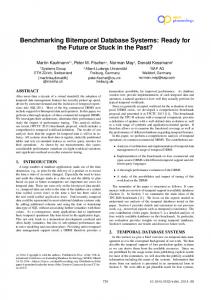
Fig. 1: Examples data graph G, pattern graph P , and resulting embeddings M1 , M2 . Instead, the problem of graph pattern matching is defined as follows: Given two graphs, G and P , where P is the smaller one, called pattern or pattern graph, the task is to compute all embeddings of P into G. Figure 1 shows an example of a graph G, a pattern graph P and all possible embeddings of P into G. In practice, we may stop the pattern matching after the first k embeddings are found. The problem of deciding whether an embedding exists is NP-complete, since a special case of this problem is to decide if a graph contains a clique of certain size, which was shown to be NP-complete [10]. However, if the pattern graph is restricted to a class of graphs of bounded treewidth, then deciding if an embedding exists is fixed-parameter tractable with respect to the size of P , i.e., exponential with respect to the size of P but polynomial with respect to the size of G [11].

3

Related Work

Related work includes theoretical foundations of graph pattern matching and benchmarks comparing different databases. Pattern Matching. Pattern match queries have gained a lot of attention recently with different extensions being introduced [12]. For example, Zou et al. [3] introduce a distance pattern match query which extends embeddings so that edges of the pattern graph are matched to paths of bounded length in the data graph. The authors demonstrate how such distance pattern match queries can be used in the analysis of friendship, author collaboration and biological networks. Fan et al. [5] introduce a graph pattern match query with regular expressions as edge constraints. Lee et al. [4] compare several state-of-the-art algorithms for solving graph pattern matching. They compare performance and scalability of algorithms such as VF2, QuickSI, GraphQL, GADDI and SPath. Each of these algorithms uses a different data structure to store graphs. We investigate how available database systems perform with regard to graph pattern matching. To the best of our knowledge, there is no experimental work on this issue. Benchmarking database systems for graph analysis. Social web and big data applications deal with highly interconnected data. Modeling this type of data in a relational database causes a high number of many-to-many relations. That is why a number of the so-called NoSQL databases have been developed [13]. Among them, graph databases are especially interesting since they often offer a proper query language. Nevertheless, since these databases are young compared to relational databases, and their query optimizers are not mature enough, it is an open question whether it is worth

4

Nataliia Pobiedina, Stefan R¨ummele, Sebastian Skritek, and Hannes Werthner

switching from a relational database to a dedicated graph database. Angles [14] outlines four types of queries on graphs: – – – –

adjacency queries, e.g., list all neighbors of a vertex; reachability queries, e.g., compute the shortest path between two nodes; pattern matching queries, which are the focus of this paper; and summarization queries, e.g., aggregate vertex or edge labels.

There are already several works comparing the performance of current database systems for graph analysis. Dominguez et al. [15] study several graph databases (Neo4j, Jena, HypergraphDB and DEX) as to their performance for reachability and summarization queries. They find that DEX and Neo4j are the most efficient databases. The other works include not only graph databases, but also relational database systems. Vicknair et al. [8] compare Neo4j, a graph database, and MySQL, a relational database, for a data provenance project. They conclude that Neo4j performs better for adjacency and reachability queries, but MySQL is considerably better for summarization queries. In the comparison they also take into account subjective measures, like maturity, level of support, ease of programming, flexibility and security. They conclude that, due to the lack of security and low maturity in Neo4j, a relational database is preferable. It is worth noting that they used Neo4j v1.0 which did not have a well developed query language and was much less mature than MySQL v5.1.42. Holzschuher and Peinl [7] show that Neo4j v1.8 is much more efficient for graph traversals than MySQL. Angles et al. [9] extend the list of considered databases and include two graph databases (Neo4j and DEX), one RDF-based database (RDF-3X), and two relational databases (Virtuoso and PostgreSQL) in their benchmark. They show that DEX and Neo4j are the best performing database systems for adjacency and reachability queries. However, none of these works consider graph pattern matching queries.

4

Benchmark for Graph Pattern Matching

Our benchmark consists of three main components: database systems, datasets and query sets. The first component includes the choice of the systems, their setup, the used data representation and encodings of pattern graphs in a specific query language. The second component consists of data graphs that are synthetically generated according to established graph models or chosen from real-world data. The last component contains the construction of pattern graphs which are then transformed into queries according to the first component and used on the datasets from the second component. 4.1

Database Systems

The database systems, which we compare, are PostgreSQL, Neo4j, Clingo, and Jena TDB. These systems have in common that they are open source and known to perform well in their respective area. But they differ considerably in the way they store data and the algorithms used to execute queries. However, all four systems allow to execute the four mentioned types of graph queries. We present in this section the data schema in each of these systems as well as the query statements in four different query languages. The used data schemas are general purpose schemas for graph representation and are not specifically tailored to graph pattern matching.

Benchmarking database systems

5

nodes

id label

edges key(source,target)

source target label

n:u0

integer

1

rdfs:label

e:0 n:u1

e:1

e:0 integer

(a) Entity relationship diagram of a graph in PostgreSQL.

n:u3

rdfs:label e:1 n:u2

0

rdfs:label

e:1 rdfs:label

0

0

(b) RDF representation for the example data graph in Figure 1.

Fig. 2: Data schema for PostreSQL and Jena TDB. PostgreSQL (SQL) PostgreSQL is an open-source object-relational database system with SQL being the query language. We use PostgreSQL server v9.1.9. The data schema we use for a graph consists of two tables: nodes and edges (see Figure 2a). The primary key of the table “nodes” is the attribute “id” and it contains an index over the attribute “label”. The attribute “label” is also indexed in the table “edges”. The attributes “source” and “target” constitute the primary key of this table. Since we are dealing with undirected graphs, the edge table contains two entries per edge. The SQL query we use to find all embeddings of the pattern graph in Figure 1 is the following: select v0.id, v1.id, v2.id from nodes v0, nodes v1, nodes v2, edges e0, edges e1 where v0.label=0 and v1.label=1 and v2.label=0 and v0.idv2.id and e0.source=v0.id and e0.target=v1.id and e0.label=0 and e1.source=v0.id and e1.target=v2.id and e1.label=1;

Listing 1.1: SQL query for the pattern graph from Figure 1. As we see, we need to do many joins for the tables “nodes” and “edges” corresponding to the amounts of vertices and edges in the pattern graph. The way the query is written, we leave it up to the database query optimizer to define the join order. It is possible to use a denormalized data schema when we have only one table which contains all information about vertices and edges. One can also manually optimize the query. However, this is not the scope of the paper. The same data schema has been used in previous benchmarking works [9, 8]. Also, our focus is at how the database engine can optimize the query execution. Such setting corresponds to a typical production scenario when an average user is not an expert. Jena TDB (SPARQL) In RDF (Resource Description Framework), entities comprise of triples (subject, predicate, object). The interpretation is that the subject applies a predicate to the object. RDF-based data can be also regarded as a graph where the subject and the object are nodes, and predicate corresponds to a link between them. There exist several RDF-based database systems. We choose Jena which is an open-source framework for building RDF based applications and provides several methods to store

6

Nataliia Pobiedina, Stefan R¨ummele, Sebastian Skritek, and Hannes Werthner

and interact with the data. For our purposes, the SPARQL server Fuseki provides the database server that is used for query answering. We use Fuseki 1.0.1, with the included Jena TDB for the persistent storage of the data. There are two main reasons for choosing TDB over SDB. Firstly, TDB was repeatedly reported to provide better performance. Secondly, especially for the comparison with PostgresSQL, it is convenient to use the native triple store TDB instead of SDB that is backed up by an SQL database. We encode the graph in RDF by representing each node of the graph as a resource (i.e., we generate an IRI for every node). The edge relation is described as properties of these resources that state to which other nodes a node is connected. Since the choice of the node that appears in the subject position of the RDF triple implies an order on the edges, we create two triples for each edge where we switch the subject and object positions. In the presence of edge labels, we introduce a separate property for each label. As a result, the structure of the RDF data resembles the original graph (cf. Figure 2b). The following query looks for embeddings of the graph pattern from Figure 1: SELECT ?X0 ?X1 ?X2 WHERE {?X0 e:0 ?X1 . ?X0 e:1 ?X2 . ?X0 a t:node . ?X0 rdfs:label ‘‘0’’ ?X1 a t:node . ?X1 rdfs:label ‘‘1’’ ?X2 a t:node . ?X2 rdfs:label ‘‘0’’ FILTER ( (?X0 6= ?X1) && (?X0 6= ?X2)

. . . && (?X1 6= ?X2))}

Listing 1.2: SPARQL query for the pattern in Figure 1 (omitting prefix definitions).

Neo4j (Cypher) Neo4j is a graph database system with Cypher being its own query language. Neo4j does not rely on a relational data layout, but a network model storage that natively stores nodes (vertices), relationships (edges) and attributes (vertex and edge labels). Neo4j has a dual free/commercial license model. We use Neo4j v1.9 which introduced considerable enhancements and optimization to the query language Cypher. It is possible to access and to modify data in Neo4j either with Cypher queries or directly via a Java API. Additionally, Neo4j can be embedded into the application or accessed via REST API. Experimental results show that Cypher via REST API performs slower than Cypher in embedded mode [7]. It is clear that queries using an embedded instance are faster than those accessing the database over the network. However, since we deploy the relational and RDF databases as servers and send queries from a client application, we also use REST API to send Cypher queries to the Neo4j server. Moreover, such a configuration models most real-world scenarios more accurately. The data schema of a graph in Neo4j corresponds to the representation in Figure 1. Vertex and edge labels are indexed with Lucene. There are several ways to express a pattern match query with Cypher. The most straightforward way is to start with matching one vertex from the pattern graph, and match all edges in one “MATCH” statement of the Cypher query. We cannot specify all vertices as the starting nodes in Cypher, since it results in a completely different set of answers. This shortcoming is unfortunate since the user is left with the task to choose the most appropriate starting node.

Benchmarking database systems

7

As an alternative, it is possible to write nested queries in Cypher. This allows to match the pattern graph one edge at a time and transfer the intermediate results to the next level: START v0 = node:my_nodes(label=’0’) MATCH v0-[e0]-v1 WHERE v1.label=1 and e0.label=0 WITH v0, v1 MATCH v0-[e1]-v2 WHERE v2.label=0 and id(v0)id(v2) and e1.label=1 RETURN id(v0), id(v1), id(v2);

Listing 1.3: Nested Cypher query for the pattern graph from Figure 1. The Neo4j developers mention that the nested queries might be especially good if the pattern graph is complicated. In both cases, straightforward and nested, we could further improve the queries by choosing more intelligently the starting node and the order in which we match the edges. Again, we do not apply these modifications since the scope of this work is on how well the database system itself can optimize the query execution. Due to space restrictions and readability issues, we report only the performance of the nested Cypher query since it shows consistently better results on our benchmark than the straightforward implementation. Clingo (ASP) Answer-set programming (ASP) is a paradigm for declarative problem solving with many applications, especially in the area of artificial intelligence (AI) and knowledge representation & reasoning (KR). In ASP a problem is modeled in the form of logic program in a way such that the so-called stable models of the program correspond to the solutions of the problem. The stable model semantics for logic programs can be computed by ASP solvers like Clingo [16], DLV [17], Smodels [18], or others. We use Clingo v4.2.1 because of its performance at various ASP competitions [19]. In database terminology, Clingo is a deductive database, supporting ASP as query language. Data is represented by facts (e.g., vertices and edges) and rules from which new facts (e.g., the embeddings) are derived. For example, the data graph from Figure 1 is given as a text file of facts in the following form. v(0, 0). v(1, 1). v(2, 0). v(3, 0). e(0, 1, 0). e(0, 2, 1). e(1, 2, 1). e(1, 3, 0). e(2, 3, 1). The first argument of the vertex predicate v indicates the node ID, the second one the label. For the edge predicate e the first two arguments represent the ID’s of the connected nodes and the third argument corresponds to the edge label: Note that we have omitted here half of the edges. To model undirected edges, we have two facts corresponding to each edge. For example, the dual version of the first edge fact above would be e(1, 0, 0). The ASP encoding for our running example is shown below: 1 {match(0,X) : v(X,0)} 1. 1 {match(1,X): e(Y,X,0)} 1 ← match(0,Y). ← match(1,X), not v(X,1). 1 {match(2,X): e(Y,X,1)} 1 ← match(0,Y). ← match(2,X), not v(X,0). ← node(K,X), node(L,X), K 6= L.

Listing 1.4: ASP query for the pattern graph from Figure 1.

8

Nataliia Pobiedina, Stefan R¨ummele, Sebastian Skritek, and Hannes Werthner

In this encoding, we derive a new binary predicate match where the first argument indicates the ID of a vertex in the pattern graph and the second argument corresponds to the ID of a vertex in the data graph. This encoding follows the “guess and check” paradigm. The match predicates are guessed as follows. The rule in Line 1 states that from all variables X such that we have a fact v(X, 0), i.e. all vertices with label 0, we choose exactly one at random for our pattern node 0. The rule in Line 2 states that from all variables X such that there exists an edge with label 0 to a node Y which we have chosen as our pattern node 0, we choose exactly one at random for our pattern node 1. Finally, we have constraints in this encoding, which basically throw away results where the guess was wrong. For example, Line 3 is such a constraint which states that a guess for variable X as our pattern node 1 is invalid if the corresponding vertex in the data graph does not have label 1. 4.2

Datasets

We use both synthetic and real data. The synthetic datasets include two types of networks: small-world and erdos renyi networks. Erdos Renyi Model (ERM) is a classical random graph model. It defines a random graph as n vertices connected by m edges, chosen randomly from the n(n − 1)/2 possible edges. The probability for edge creation is given by the parameter p. We use parameter p = 0.01. This graph is connected. Preferential Attachment Model (PAM), or small-world model, grows a graph of n nodes by attaching new nodes each with m edges that are preferentially attached to existing nodes with high degree. We use m = 4. We choose this graph generation model, since it has been shown that many real-world networks follow this model [20]. In both cases, we generate graphs with 1000 and 10,000 nodes. Vertex labels are assigned randomly. We do not produce edge labels for the synthetic datasets. The real-world datasets include a citation network and a terrorist organization collaboration network. The terrorist organization collaboration network (GTON) is constructed on the basis of Global Terrorism Database3 which contains 81,800 worldwide terrorist attack events in the last 40 years. In this network, each vertex represents a terrorist organization, and edges correspond to the collaboration of organizations in the common attacks. Vertices are assigned two labels according to the number of recorded events: either 0 if the organization conducted less than 2 attacks, or 1 otherwise. Edges have also two labels depending on the amount of common attacks: either 0 if two organizations collaborated less than twice, or 1 in the other case. The citation network (HepTh) covers arXiv papers from the years 1992–2003 which are categorized as High Energy Physics Theory. This dataset was part of the KDD Cup 2003 [21]. In this network, a vertex corresponds to a scientific publication. An edge between two vertices indicates that one of the papers cites the second one. We ignore the direction of the citation, and consider the network undirected. As vertex labels, we use the grouped number of authors of the corresponding paper. The edge label corresponds to the absolute difference between publication years of the adjacent vertices. We summarize the statistics of the constructed data graphs in Table 1. 3

http://www.start.umd.edu/gtd

Benchmarking database systems

9

Table 1: Summary of the datasets. Synthetic data ERM 1000 ERM 10000 PAM 1000 PAM 10000 # vertices 1,000 10,000 1,000 10,000 # edges 4,890 500,065 3,984 39,984 avg degree 9.78 100.01 7.97 8 max degree 22 143 104 298 # vertex labels 2 2 2 2 # edge labels − − − − Dataset

4.3

Real data GTON HepTh 335 9,162 335 52,995 1.98 11.57 13 430 2 5 2 5

Query Sets

We produce two sets of pattern graphs which are then used in graph pattern matching queries. All the generated pattern graphs are connected. The first set is generated synthetically with a procedure which takes as input the number of vertices and number of edges. The queries in this set have only vertex labels. In the first run of the procedure, we generate queries with five vertices and vary the number of edges from 4 till 10. In the second run, we fix the number of edges to ten and vary the number of vertices from 5 till 11. We generate 20 pattern graphs for each parameter configuration in both cases. We construct the synthetic queries this way in order to verify how the performance of database systems is influenced by the size of the pattern graph: first, we focus on the dependence on the number of edges, and second, on the number of vertices. We call this set of pattern graphs synthetic patterns. The second set of queries is generated specifically for real-world data using graph pattern mining. Thereby we look for patterns which occur at least five times in our data graphs. In this set we specify not only vertex labels but also edge labels. The reason for this set of queries is twofold. First, we can study the performance on pattern graphs with guaranteed embeddings. Second, frequent graph pattern mining is a typical application scenario for graph pattern matching [12]. For example, graph pattern mining together with matching is used to predict citation counts for HepTh dataset in [22].

5

Experimental Results

Experimental setup. The server and the client application are hosted on the same 64 bit Linux machine. It has four AMD Opteron CPUs at 2.4GHz and 8GB of RAM. The client application is written in Python and uses wrappers to connect to the database systems. The warm-up procedure for PostgreSQL, SPARQL and Neo4j consists of executing several pattern match queries. Since the problem at hand is NP-complete, we limit the execution time for all queries and database systems to three minutes to avoid longlasting queries and abnormal memory consumption. We use the same order of edges in pattern graphs when encoding them into queries in different database languages. Except for our smallest dataset, GTON, we query only for the first 1000 embeddings. As Lee et al. [4] point out, this limit on embeddings is reasonable in practice. We would like to stress that all systems provide correct answers and agree on the number of discovered embeddings.

10

Nataliia Pobiedina, Stefan R¨ummele, Sebastian Skritek, and Hannes Werthner

Synthetic data. We report the performance of the database systems for synthetic queries on the four synthetic datasets in Figures 3 and 4. The performance of PostgreSQL is labeled by “SQL”. The label “Cypher” stands for the nested Cypher query. Label “SPARQL” and “ASP” show the performance of Jena TDB and Clingo correspondingly. The performance is measured in terms of the execution time per query, and we plot the execution times on a logarithmic scale for better visualization. We also consider how many queries the database system manages to execute within three minutes. Charts (a) and (c) in the figures correspond to the case where we use pattern graphs with five vertices and change the number of edges from four till ten. We have 20 distinct queries for each category, this means each data point corresponds to the average execution time over 20 queries. Since we consider only connected patterns, all patterns with five vertices and four edges are acyclic. With increasing number of edges, the number of cycles in patterns increases. Patterns with ten edges are complete graphs. Moreover, for these patterns the principle of containment holds: pattern graphs with less edges are subgraphs to some pattern graphs with more edges. Hence, the number of found embeddings can only drop or remain the same as we increase the number of edges. In charts (b) and (d) from Figures 3 and 4 we start with the same complete pattern graphs as in the last category in charts (a) and (c). Then, by fixing the number of edges to 10, we increase the number of vertices till 11. Pattern graphs with 11 vertices and 10 edges are again acyclic graphs. By construction, the principle of containment does not hold here. Hence, in charts (a) and (c) we investigate how the increasing number of edges influences the performance of the database systems. For charts (b) and (d), the focus is on the dependence between the number of vertices and execution time. Another aspect studied is the scalability of the database systems with regard to the size of the data graph. Thus, in Figures 3 and 4 charts (a) and (b) correspond to smaller graphs while charts (c) and (d) show results for bigger ones. Since we observe that the performance of the systems also depends on the structure of the pattern, we present the dependence of the run time on the number of cycles in the pattern in Figure 5. The results indicate that SPARQL is on average better than the others. We observe that the performance of the database systems depends on the following factors: (I) size of the data graph; (II) size of the pattern graph; and (III) structure of the pattern graph. PostgreSQL shows incoherent results. For example, we can observe a peak in the average run time for the pattern graphs with five vertices and six edges for small datasets in PostgreSQL (see Figure 3a,4a). One reason for this behavior is that in some cases the query optimizer fails in determining the best join strategy (we recall that PostgreSQL offers nested loop-, hash-, and merge join). For example, by disabling the usage of the nested loop join in the configuration of PostgreSQL, we arrive at an average run time of two seconds instead of eight for the dataset PAM1000 for synthetic patterns. However, this trick works only for the smaller graphs. Overall, PostgreSQL does not scale with regard to the size of the pattern graph. We can see it especially in Figure 3b. Furthermore, none of the queries in Figure 3d finished within 3 minutes. Surprisingly, SPARQL shows the best performance in almost all cases. This complements previous works ([9] and [15]) where RDF-based systems are among the worst performing systems for the tasks of graph analysis, except our case of graph pattern matching. Our understanding is that, besides solving a different problem, the authors

Benchmarking database systems

11

(a) Patterns with 5 vertices and varying number (b) Patterns with 10 edges and varying number of edges for ERM1000. of vertices for ERM1000.

(c) Patterns with 5 vertices and varying number (d) Patterns with 10 edges and varying number of vertices for ERM10000. of edges for ERM10000.

Fig. 3: Average run time in seconds on logarithmic scale for ERM. use native access to Neo4j in [15], and access to Neo4j through Cypher via REST API has been shown to be much slower [7]. Also, Renzo et al. [9] chose RDF-3X which seems to perform worse than Jena TDB. Like PostgreSQL, Jena TDB shows incoherence, e.g., there is a peak in average run time for patterns with five vertices and six edges (see Figures 3a and 4a). In Figure 5 we observe that SPARQL can handle pattern graphs with two cycles considerably worse than the others. It seems that the query optimizer of Jena TDB makes worse choices for the matching order of edges, however, it is unclear if such behavior can be configured since the query optimizer is not transparent. Though SPARQL shows better run times, it cannot handle efficiently complete patterns on ERM10000 like the other database systems (see Figure 3d). SPARQL turned out to be very sensitive towards the changes in the data schema. If we put edges as resources in Jena TDB, it becomes the worst performing database system. Such change in the data schema might be relevant if we introduce more than one property for the edges or we have a string property associated with the edges. At the same time, such drastic changes to the data schema are not required for the other database systems. Our results show that Clingo is not a scalable system with regard to the size of the data graph. It cannot execute any query for cyclic patterns within three minutes on ERM with 10000 vertices (Figure 3c,3d), but can only handle acyclic patterns on these datasets. Though the size of the pattern affects the run time of Clingo, the decrease in the run time happens mainly due to the growth of cycles in the pattern graph (Figure 5). Like for Clingo, cyclic patterns pose the main problem for Neo4j. The average run times grow with the increase of the number of edges in charts (a) and (c), and then drop

12

Nataliia Pobiedina, Stefan R¨ummele, Sebastian Skritek, and Hannes Werthner

(a) Patterns with 5 vertices and varying number (b) Patterns with 10 edges and varying number of vertices for PAM1000. of edges for PAM1000.

(c) Patterns with 5 vertices and varying number (d) Patterns with 10 edges and varying number of edges for PAM10000. of vertices for PAM10000.

Fig. 4: Average run time in seconds on logarithmic scale for PAM. with the increase of the number of vertices in charts (b) and (d) in Figures 3 and 4. Thus, the worst run time is for complete patterns. This trend is illustrated in Figure 5. Unlike ASP, the dependence between the run time and number of cycles is not linear for Cypher. The issue is that both Cypher and ASP rely on backtracking algorithms. Hence, the starting vertex in the queries is very important for the performance. We could further optimize the queries by choosing the vertex with the least frequent label as the starting point. This change is especially crucial for Neo4j, since its query optimizer is not as mature as the one for PostgreSQL or Clingo. When analyzing the change of average run times between the small and big data graphs in each figure, we see that the performance of ASP drastically drops while Cypher shows the least change in performance among the considered systems. This trend is especially clear for ERM (Figure 3). As mentioned, database systems not always manage to execute our queries within three minutes. PostgreSQL finishes not all queries with 10 edges on the small PAM and ERM graphs within the time limit. Especially problems arise with patterns which have more than 9 vertices. For example, PostgreSQL finishes only two queries out of 20 on the small PAM graph for pattern graphs with 10 edges and 11 vertices. Furthermore, on both big graphs (PAM10000 and ERM10000) PostgreSQL can execute only a fraction of queries for pattern graphs with more than six edges. Clingo, Neo4j and SPARQL execute all queries for acyclic patterns within the established time limit irrelevant of the size of data and pattern graphs. An interesting observation is that Clingo either executes all queries within the specified category, or none at all. While Neo4j can handle more cyclic patterns compared to Clingo, the number of executed queries within three minutes still drops with the increase of the number of cycles.

Benchmarking database systems

13

(a) Patterns with 5 vertices and varying num- (b) Patterns with 10 edges and varying number ber of cycles. of cycles.

Fig. 5: Average run time in seconds on log-scale for synthetic patterns on PAM1000. Real world data. Synthetic patterns do not have edge labels, and for many of them no embedding exists in the data graphs. Therefore, we construct another set of patterns by ensuring that each of them occurs at least 5 times in the dataset. Hence, the sets of generated patterns differ for GTON and HepTh. In both cases graph patterns have from 5 up to 10 edges, and almost all of them are acyclic. More precisely, the generated patterns have either the same number of vertices as edges, or they have one vertex more than edges. The performance for this setting is shown in Figure 6. Again, we use 20 pattern graphs in each category, which corresponds to a data point in the charts, and report the average run time for each category on the logarithmic scale in the figure. Clingo and Jena TDB show equally good performance on our smallest dataset GTON (Figure 6a) with Clingo being better for the bigger pattern graphs. Neo4j and PostgreSQL are considerably worse in this case. However, ASP drops in its performance on the dataset HepTh (Figure 6b). Clingo does not use any indexes on labels and has no caching mechanism. This leads to a considerable drop in the performance when the data graph is especially big. At the same time, SPARQL shows the best run times on the bigger dataset, though compared to GTON the run times increase. Surprisingly, PostgreSQL does not provide the best performing results in any case on the real-world data. We can observe a clear trend that the average run time for PostgreSQL considerably grows with the increase of the number of edges in the pattern graphs. Moreover, PostgreSQL executes only five queries out of 20 for pattern graph with 7 edges on HepTh. This observation proves once again that PostgreSQL does not scale with regard to the size of the pattern graphs. Since the more edges there are in the pattern graph, the more joins for tables PostgreSQL has to do. In terms of scalability with the size of the data graph, we conclude that Neo4j shows the best results. Judging from the results on GTON, we may conclude that there is a lot of space for improvement for Neo4j. We believe that the query optimizer in Neo4j could be tuned to narrow the gap between Cypher and SPARQL in this case. Summary. As a result, we can provide the following insights. In general, Jena TDB is better for graph pattern matching with regard to the data schema provided in our benchmark. If we have a very small data graph, Clingo is a good choice. If we have a big data graph and pattern graphs are mainly acyclic, Neo4j provides good results. However, in case of big data graphs and cyclic pattern graphs with more than seven edges, none of the studied database systems perform well.

14

Nataliia Pobiedina, Stefan R¨ummele, Sebastian Skritek, and Hannes Werthner

(a) Frequent pattern queries for GTON.

(b) Frequent pattern queries for HepTh.

Fig. 6: Average run time in seconds on logarithmic scale for GTON and HepTH.

6

Conclusion and Future Work

We have studied how four database systems perform with regard to the problem of graph pattern matching. In our study we use a relational database PostgreSQL, a graph database Neo4j, a deductive database Clingo and RDF-based database Jena TDB. The most mature system among these four is PostgreSQL with Neo4j being the youngest. By conducting extensive experiments on synthetic and real-world datasets we come to the following conclusions. Clingo does not scale with the size of the data graph. Its performance drastically drops when the data graph becomes bigger. Though the performance of Clingo is not much influenced by the size of the pattern graph, it worsens with the growth of the cycles in the pattern graph. Neo4j cannot efficiently handle cyclic pattern graphs. However, it scales very well with regard to the size of the data graph as well as the size of the pattern graph. The performance of PostgreSQL oscillates generally due to the changes in the join order chosen in the execution plan. Though PostgreSQL shows good performance for cyclic patterns, it does not scale well with regard to the size of the pattern graphs and the size of the data graphs. Jena TDB is in general better than the other database systems on our benchmark. However, it turned out to be the most sensitive system to the changes in the data schema. In our opinion, the efficiency of databases for solving graph pattern matching tasks is not yet good enough for information systems that deal with real-world big data scenarios. The database systems should consider implementing the state-of-the-art algorithms for this task [4]. For example, the query optimizer of Neo4j cannot ensure the most optimal choice of the starting node, and of the join order for the edges and vertices. The latter holds also for PostgreSQL which can be optimized by tuning up the configuration settings of the server. Furthermore, in all database systems we can configure the servers to achieve better results, but it is unclear what is the best configuration if we need to perform a variety of graph queries and not just graph pattern matching. This calls for further investigation. We plan to investigate how the efficiency can be increased by influencing the matching order of the edges. Future work includes the integration of other types of graph queries into our benchmark.

Benchmarking database systems

15

References 1. Bringmann, B., Berlingerio, M., Bonchi, F., Gionis, A.: Learning and predicting the evolution of social networks. IEEE Intelligent Systems 25(4) (2010) 26–35 2. Asnar, Y., Paja, E., Mylopoulos, J.: Modeling design patterns with description logics: A case study. In: Proc. CAiSE. (2011) 169–183 ¨ 3. Zou, L., Chen, L., Ozsu, M.T., Zhao, D.: Answering pattern match queries in large graph databases via graph embedding. VLDB J. 21(1) (2012) 97–120 4. Lee, J., Han, W.S., Kasperovics, R., Lee, J.H.: An in-depth comparison of subgraph isomorphism algorithms in graph databases. PVLDB 6(2) (2012) 133–144 5. Fan, W., Li, J., Ma, S., Tang, N., Wu, Y.: Adding regular expressions to graph reachability and pattern queries. Frontiers of Computer Science 6(3) (2012) 313–338 6. Xu, J., Chen, H.: Criminal network analysis and visualization. Commun. ACM 48(6) (2005) 100–107 7. Holzschuher, F., Peinl, R.: Performance of graph query languages: comparison of Cypher, Gremlin and native access in Neo4j. In: Proc. EDBT/ICDT Workshops. (2013) 195–204 8. Vicknair, C., Macias, M., Zhao, Z., Nan, X., Chen, Y., Wilkins, D.: A comparison of a graph database and a relational database: a data provenance perspective. In: Proc. ACM Southeast Regional Conference. (2010) 42 9. Angles, R., Prat-P´erez, A., Dominguez-Sal, D., Larriba-Pey, J.L.: Benchmarking database systems for social network applications. In: Proc. GRADES. (2013) 15 10. Karp, R.M.: Reducibility among combinatorial problems. In: Proc. Complexity of Computer Computations. (1972) 85–103 11. Alon, N., Yuster, R., Zwick, U.: Color-coding. J. ACM 42(4) (1995) 844–856 12. Gallagher, B.: Matching structure and semantics: A survey on graph-based pattern matching. In: Proc. AAAI Fall Symposium on Capturing and Using Patterns for Evidence Detection. (2006) 13. Tudorica, B.G., Bucur, C.: A comparison between several NoSQL databases with comments and notes. In: Proc. Roedunet International Conference. (2011) 1–5 14. Angles, R.: A comparison of current graph database models. In: Proc. ICDE Workshops. (2012) 171–177 15. Dominguez-Sal, D., Urb´on-Bayes, P., Gim´enez-Va˜no´ , A., G´omez-Villamor, S., Mart´ınezBazan, N., Larriba-Pey, J.L.: Survey of graph database performance on the HPC scalable graph analysis benchmark. In: Proc. WAIM Workshops. (2010) 37–48 16. Gebser, M., Kaufmann, B., Kaminski, R., Ostrowski, M., Schaub, T., Schneider, M.T.: Potassco: The Potsdam answer set solving collection. AI Commun. 24(2) (2011) 107–124 17. Leone, N., Pfeifer, G., Faber, W., Eiter, T., Gottlob, G., Perri, S., Scarcello, F.: The DLV system for knowledge representation and reasoning. ACM Trans. Comput. Log. 7(3) (2006) 499–562 18. Syrj¨anen, T., Niemel¨a, I.: The Smodels system. In: Proc. LPNMR. (2001) 434–438 19. Alviano, M., et al.: The fourth answer set programming competition: Preliminary report. In: Proc. LPNMR. (2013) 42–53 20. Barab´asi, A.L., Albert, R.: Emergence of scaling in random networks. Science Magazine 286(5439) (1999) 509–512 21. Gehrke, J., Ginsparg, P., Kleinberg, J.M.: Overview of the 2003 KDD cup. SIGKDD Explorations 5(2) (2003) 149–151 22. Pobiedina, N., Ichise, R.: Predicting citation counts for academic literature using graph pattern mining. In: Proc. IEA/AIE. (2014) 109–119