Beyond CCA: Moment Matching for Multi-View Models - arXiv

Beyond CCA: Moment Matching for Multi-View Models

arXiv:1602.09013v2 [stat.ML] 3 Jun 2016

Anastasia Podosinnikova Francis Bach Simon Lacoste-Julien ´ INRIA - Ecole normale supérieure, Paris

Abstract We introduce three novel semi-parametric extensions of probabilistic canonical correlation analysis with identifiability guarantees. We consider moment matching techniques for estimation in these models. For that, by drawing explicit links between the new models and a discrete version of independent component analysis (DICA), we first extend the DICA cumulant tensors to the new discrete version of CCA. By further using a close connection with independent component analysis, we introduce generalized covariance matrices, which can replace the cumulant tensors in the moment matching framework, and, therefore, improve sample complexity and simplify derivations and algorithms significantly. As the tensor power method or orthogonal joint diagonalization are not applicable in the new setting, we use non-orthogonal joint diagonalization techniques for matching the cumulants. We demonstrate performance of the proposed models and estimation techniques on experiments with both synthetic and real datasets.

1. Introduction Canonical correlation analysis (CCA), originally introduced by Hotelling (1936), is a common statistical tool for the analysis of multi-view data. Examples of such data include, for instance, representation of some text in two languages (e.g., Vinokourov et al., 2002) or images aligned with text data (e.g., Hardoon et al., 2004; Gong et al., 2014). Given two multidimensional variables (or datasets), CCA finds two linear transformations (factor loading matrices) that mutually maximize the correlations between the transformed variables (or datasets). Together with its kernelized version (see, e.g., Shawe-Taylor & Cristianini, Proceedings of the 33 rd International Conference on Machine Learning, New York, NY, USA, 2016. JMLR: W&CP volume 48. Copyright 2016 by the author(s).

ANASTASIA . PODOSINNIKOVA @ INRIA . FR FRANCIS . BACH @ INRIA . FR FIRSTNAME . LASTNAME @ INRIA . FR

2004; Bach & Jordan, 2003), CCA has a wide range of applications (see, e.g., Hardoon et al. (2004) for an overview). Bach & Jordan (2005) provide a probabilistic interpretation of CCA: they show that the maximum likelihood estimators of a particular Gaussian graphical model, which we refer to as Gaussian CCA, is equivalent to the classical CCA by Hotelling (1936). The key idea of Gaussian CCA is to allow some of the covariance in the two observed variables to be explained by a linear transformation of common independent sources, while the rest of the covariance of each view is explained by their own (unstructured) noises. Importantly, the dimension of the common sources is often significantly smaller than the dimensions of the observations and, potentially, than the dimensions of the noise. Examples of applications and extensions of Gaussian CCA are the works by Socher & Fei-Fei (2010), for mapping visual and textual features to the same latent space, and Haghighi et al. (2008), for machine translation applications. Gaussian CCA is subject to some well-known unidentifiability issues, in the same way as the closely related factor analysis model (FA; Bartholomew, 1987; Basilevsky, 1994) and its special case, the probabilistic principal component analysis model (PPCA; Tipping & Bishop, 1999; Roweis, 1998). Indeed, as FA and PPCA are identifiable only up to multiplication by any rotation matrix, Gaussian CCA is only identifiable up to multiplication by any invertible matrix. Although this unidentifiability does not affect the predictive performance of the model, it does affect the factor loading matrices and hence the interpretability of the latent factors. In FA and PPCA, one can enforce additional constraints to recover unique factor loading matrices (see, e.g., Murphy, 2012). A notable identifiable version of FA is independent component analysis (ICA; Jutten, 1987; Jutten & Hérault, 1991; Comon & Jutten, 2010). One of our goals is to introduce identifiable versions of CCA. The main contributions of this paper are as follows. We first introduce for the first time, to the best of our knowledge, three new formulations of CCA: discrete, non-Gaussian, and mixed (see Section 2.1). We then provide identifiability guarantees for the new models (see Section 2.2). Then,


in order to use a moment matching framework for estimation, we first derive a new set of cumulant tensors for the discrete version of CCA (Section 3.1). We further replace these tensors with their approximations by generalized covariance matrices for all three new models (Section 3.2). Finally, as opposed to standard approaches, we use a particular type of non-orthogonal joint diagonalization algorithms for extracting the model parameters from the cumulant tensors or their approximations (Section 4). Models. The new CCA models are adapted to applications where one or both of the data-views are either counts, like in the bag-of-words representation for text, or continuous data, for instance, any continuous representation of images. A key feature of CCA compared to joint PCA is the focus on modeling the common variations of the two views, as opposed to modeling all variations (including joint and marginal ones). Moment matching. Regarding parameter estimation, we use the method of moments, also known as “spectral methods.” It recently regained popularity as an alternative to other estimation methods for graphical models, such as approximate variational inference or MCMC sampling. Estimation of a wide range of models is possible within the moment matching framework: ICA (e.g., Cardoso & Comon, 1996; Comon & Jutten, 2010), mixtures of Gaussians (e.g., Arora & Kannan, 2005; Hsu & Kakade, 2013), latent Dirichlet allocation and topic models (Arora et al., 2012; 2013; Anandkumar et al., 2012; Podosinnikova et al., 2015), supervised topic models (Wang & Zhu, 2014), Indian buffet process inference (Tung & Smola, 2014), stochastic languages (Balle et al., 2014), mixture of hidden Markov models (Sübakan et al., 2014), neural networks (see, e.g., Anandkumar & Sedghi, 2015; Janzamin et al., 2016), and other models (see, e.g., Anandkumar et al., 2014, and references therein). Moment matching algorithms for estimation in graphical models mostly consist of two main steps: (a) construction of moments or cumulants with a particular diagonal structure and (b) joint diagonalization of the sample estimates of the moments or cumulants to estimate the parameters. Cumulants and generalized covariance matrices. By using the close connection between ICA and CCA, we first derive in Section 3.1 the cumulant tensors for the discrete version of CCA from the cumulant tensors of a discrete version of ICA (DICA) proposed by Podosinnikova et al. (2015). Extending the ideas from the ICA literature (Yeredor, 2000; Todros & Hero, 2013), we further generalize in Section 3.2 cumulants as the derivatives of the cumulant generating function. This allows us to replace cumulant tensors with “generalized covariance matrices”, while preserving the rest of the framework. As a consequence of working with the second-order information only, the

derivations and algorithms get significantly simplified and the sample complexity potentially improves. Non-orthogonal joint diagonalization. When estimating model parameters, both CCA cumulant tensors and generalized covariance matrices for CCA lead to non-symmetric approximate joint diagonalization problems. Therefore, the workhorses of the method of moments in similar context — orthogonal diagonalization algorithms, such as the tensor power method (Anandkumar et al., 2014), and orthogonal joint diagonalization (Bunse-Gerstner et al., 1993; Cardoso & Souloumiac, 1996) — are not applicable. As an alternative, we use a particular type of non-orthogonal Jacobilike joint diagonalization algorithms (see Section 4). Importantly, the joint diagonalization problem we deal with in this paper is conceptually different from the one considered, e.g., by Kuleshov et al. (2015) (and references therein) and, therefore, the respective algorithms are not applicable here.

2. Multi-view models 2.1. Extensions of Gaussian CCA Gaussian CCA. Classical CCA (Hotelling, 1936) aims to find projections D1 ∈ RM1 ×K and D2 ∈ RM2 ×K , of two observation vectors x1 ∈ RM1 and x2 ∈ RM2 , each representing a data-view, such that the projected data, D1> x1 and D2> x2 , are maximally correlated. Similarly to classical PCA, the solution boils down to solving a generalized SVD problem. The following probabilistic interpretation of CCA is well known (Browne, 1979; Bach & Jordan, 2005; Klami et al., 2013). Given that K sources are i.i.d. standard normal random variables, α ∼ N (0, IK ), the Gaussian CCA model is given by x1 | α, µ1 , Ψ1 ∼ N (D1 α + µ1 , Ψ1 ), x2 | α, µ2 , Ψ2 ∼ N (D2 α + µ2 , Ψ2 ),

(1)

where the matrices Ψ1 ∈ RM1 ×M1 and Ψ2 ∈ RM2 ×M2 are positive semi-definite. Then, the maximum likelihood solution of (1) coincides (up to permutation, scaling, and multiplication by any invertible matrix) with the classical CCA solution. The model (1) is equivalent to x1 = D 1 α + ε1 , x2 = D 2 α + ε2 ,

(2)

where the noise vectors are normal random variables, i.e. ε1 ∼ N (µ1 , Ψ1 ) and ε2 ∼ N (µ2 , Ψ2 ), and the following independence assumptions are made: α1 , . . . , αK are mutually independent, α ⊥⊥ ε1 , ε2

and

ε1 ⊥⊥ ε2 .

(3)

The following three models are our novel semi-parametric extensions of Gaussian CCA (1)–(2).


K

ε1

ε2

αk

of the covariance matrices of the noises of the models (4)– (6). The following example illustrates the mentioned relation. Assuming a linear structure for the noise, (non-) Gaussian CCA (NCCA) takes the form x1 = D1 α + F1 β1 ,

x1m N

M1

x2m M2

D1

D2

Figure 1. Graphical models for non-Gaussian (4), discrete (5), and mixed (6) CCA.

Multi-view models. The first new model follows by dropping the Gaussianity assumption on α, ε1 , and ε2 . In particular, the non-Gaussian CCA model is defined as x1 = D1 α + ε1 , (4) x2 = D2 α + ε2 , where, as opposed to (2), no assumptions are made on the sources α and the noise ε1 and ε2 except for the independence assumption (3). Similarly to Podosinnikova et al. (2015), we further “discretize” non-Gaussian CCA (4) by applying the Poisson distribution to each view (independently on each variable): x1 | α, ε1 ∼ Poisson(D1 α + ε1 ), (5) x2 | α, ε2 ∼ Poisson(D2 α + ε2 ). We obtain the (non-Gaussian) discrete CCA (DCCA) model, which is adapted to count data (e.g., such as word counts in the bag-of-words model of text). In this case, the sources α, the noise ε1 and ε2 , and the matrices D1 and D2 have non-negative components. Finally, by combining non-Gaussian and discrete CCA, we also introduce the mixed CCA (MCCA) model: x1 = D1 α + ε1 , (6) x2 | α, ε2 ∼ Poisson(D2 α + ε2 ), which is adapted to a combination of discrete and continuous data (e.g., such as images represented as continuous vectors aligned with text represented as counts). Note that no assumptions are made on distributions of the sources α except for independence (3). The plate diagram for the models (4)–(6) is presented in Fig. 1. We call D1 and D2 factor loading matrices (see a comment on this naming convention in Appendix A.2). Relation between PCA and CCA. The key difference between Gaussian CCA and the closely related FA/PPCA models is that the noise in each view of Gaussian CCA is not assumed to be isotropic unlike for FA/PPCA. In other words, the components of the noise are not assumed to be independent or, equivalently, the noise covariance matrix does not have to be diagonal and may exhibit a strong structure. In this paper, we never assume any diagonal structure

x2 = D2 α + F2 β2 ,

(7)

where ε1 = F1 β1 with β1 ∈ RK1 and ε2 = F2 β2 with β2 ∈ RK2 . By stacking the vectors on the top of each other   α x1 D1 F1 0 x= , D= , z = β1  , (8) x2 D2 0 F2 β2 we rewrite the model as x = Dz. Assuming that the noise sources β1 and β2 have mutually independent components, ICA is recovered. If the sources z are further assumed to be Gaussian, x = Dz corresponds to PPCA. However, we do not assume the noise in Gaussian CCA (and in (4)–(6)) to have a very specific low dimensional structure. Related work. Some extensions of Gaussian CCA were proposed in the literature: exponential family CCA (Virtanen, 2010; Klami et al., 2010) and Bayesian CCA (see, e.g., Klami et al., 2013, and references therein). Although exponential family CCA can also be discretized, it assumes in practice that the prior of the sources is a specific combination of Gaussians. Bayesian CCA models the factor loading matrices and the covariance matrix of Gaussian CCA. Sampling or approximate variational inference are used for estimation and inference in both models. Both models, however, lack our identifiability guarantees and are quite different from the models (4)–(6). Song et al. (2014) consider a multi-view framework to deal with non-parametric mixture components, while our approach is semi-parametric with an explicit linear structure (our loading matrices) and makes the explicit link with CCA. See also Ge & Zou (2016) for a related approach. 2.2. Identifiability In this section, the identifiability of the factor loading matrices D1 and D2 is discussed. In general, for the type of models considered, the unidentifiability to permutation and scaling cannot be avoided. In practice, this unidentifiability is however easy to handle and, in the following, we only consider identifiability up to permutation and scaling. ICA can be seen as an identifiable analog of FA/PPCA. Indeed, it is known that the mixing matrix D of ICA is identifiable if at most one source is Gaussian (Comon, 1994). The factor loading matrix of FA/PPCA is unidentifiable since it is defined only up to multiplication by any orthogonal rotation matrix. Similarly, the factor loading matrices of Gaussian CCA (1), which can be seen as a multi-view extension of PPCA, are


identifiable only up to multiplication by any invertible matrix (Bach & Jordan, 2005). We show the identifiability results for the new models (4)–(6): the factor loading matrices of these models are identifiable if at most one source is Gaussian (see Appendix B for a proof). Theorem 1. Assume that matrices D1 ∈ RM1 ×K and D2 ∈ RM2 ×K , where K ≤ min(M1 , M2 ), have full rank. If the covariance matrices cov(x1 ) and cov(x2 ) exist and if at most one source αk , for k = 1, . . . , K, is Gaussian and none of the sources are deterministic, then the models (4)– (6) are identifiable (up to scaling and joint permutation). Importantly, the permutation unidentifiability does not destroy the alignment in the factor loading matrices, that is, for some permutation matrix P , if D1 P is the factor loading matrix of the first view, than D2 P must be the factor loading matrix of the second view. This property is important for the interpretability of the factor loading matrices and, in particular, is used in our experiments in Section 5.

cov(x) = E[cov(x|y)] + cov[E(x|y), E(x|y)] = diag[E(y)] + cov(y), since all the cumulants of a Poisson random variable with parameter y are equal to y. Therefore, S = cov(y). Similarly, by the law of total cumulance T = cum(y). Then, by the multilinearity property for cumulants, one obtains S = D cov(α)D> , (11) T = cum(α) ×1 D> ×2 D> ×3 D> , where ×i denotes the i-mode tensor-matrix product (see, e.g., Kolda & Bader, 2009). Since the covariance cov(α) and cumulant cum(α) of the independent sources are diagonal, (11) is called the diagonal form. This diagonal form is further used for estimation of D (see Section 4). Noisy discrete ICA. The following noisy version (12) of the DICA model reveals the connection between DICA and DCCA. Noisy discrete ICA is obtained by adding nonnegative noise ε, such that α ⊥⊥ ε, to discrete ICA (9): x | α, ε ∼ Poisson (Dα + ε) .

3. The cumulants and generalized covariances In this section, we first derive the cumulant tensors for the discrete CCA model (Section 3.1) and then generalized covariance matrices (Section 3.2) for the models (4)–(6). We show that both cumulants and generalized covariances have a special diagonal form and, therefore, can be efficiently used within the moment matching framework (Section 4).

In this section, we derive the DCCA cumulants as an extension of the cumulants of discrete independent component analysis (DICA; Podosinnikova et al., 2015). Discrete ICA. Podosinnikova et al. (2015) consider the discrete ICA model (9), where x ∈ RM has conditionally independent Poisson components with mean Dα and α ∈ RK has independent non-negative components: x | α ∼ Poisson(Dα).

Let y := Dα + ε and S and T are defined as in (10). Then a simple extension of the derivations from above gives S = cov(y) and T = cum(y). Since the covariance matrix (cumulant tensor) of the sum of two independent multivariate random variables, Dα and ε, is equal to the sum of the covariance matrices (cumulant tensors) of these variables, the “perturbed” version of the diagonal form (11) follows S = Dcov(α)D> + cov(ε),

3.1. From discrete ICA to discrete CCA

(9)

For estimating the factor loading matrix D, Podosinnikova et al. (2015) propose an algorithm based on the moment matching method with the cumulants of the DICA model. In particular, they define the DICA S-covariance matrix and T-cumulant tensor as S := cov(x) − diag [Ex] , (10) [T ]m1 m2 m3 := cum(x)m1 m2 m3 + [τ ]m1 m2 m3 , where indices m1 , m2 , and m3 take the values in 1, . . . , M , and [τ ]m1 m2 m3 = 2δm1 m2 m3 Exm1 −δm2 m3 cov(x)m1 m2 − δm1 m3 cov(x)m1 m2 − δm1 m2 cov(x)m1 m3 with δ being the Kronecker delta. For completeness, we outline the derivation by Podosinnikova et al. (2015) below. Let y := Dα. By the law of total expectation E(x) = E(x|y) = E(y) and by the law of total covariance

(12)

T = cum(α) ×1 D> ×2 D> ×3 D> + cum(ε).

(13)

DCCA cumulants. By analogy with (8), stacking the observations x = [x1 ; x2 ], the factor loading matrices D = [D1 ; D2 ], and the noise vectors ε = [ε1 ; ε2 ] of discrete CCA (5) gives a noisy version of discrete ICA with a particular form of the covariance matrix of the noise: cov(ε1 ) 0 cov(ε) = , (14) 0 cov(ε2 ) which is due to the independence ε1 ⊥⊥ ε2 . Similarly, the cumulant cum(ε) of the noise has only two diagonal blocks which are non-zero. Therefore, considering only those parts of the S-covariance matrix and T-cumulant tensor of noisy DICA that correspond to zero blocks of the covariance cov(ε) and cumulant cum(ε), gives immediately a matrix and tensor with a diagonal structure similar to the one in (11). Those blocks are the cross-covariance and cross-cumulants of x1 and x2 . We define the S-covariance matrix of discrete CCA1 as the cross-covariance matrix of x1 and x2 : S12 := cov(x1 , x2 ). (15) 1

Note that S21 := cov(x2 , x1 ) is just the transpose of S12 .


From (13) and (14), the matrix S12 has the following diagonal form S12 = D1 cov(α)D2> . (16) Similarly, we define the T-cumulant tensors of discrete CCA ( T121 ∈ RM1 ×M2 ×M1 and T122 ∈ RM1 ×M2 ×M2 ) through the cross-cumulants of x1 and x2 , for j = 1, 2: [T12j ]m1 m2 m ˜j ˜ j := [cum(x1 , x2 , xj )]m1 m2 m − δmj m ˜ j [cov(x1 , x2 )]m1 m2 ,

(17)

where the indices m1 , m2 , and m ˜ j take the values m1 ∈ 1, . . . , M1 , m2 ∈ 1, . . . , M2 , and m ˜ j ∈ 1, . . . , Mj . From (11) and the mentioned block structure (14) of cov(ε), the DCCA T-cumulants have the diagonal form: T121 = cum(α) ×1 D1> ×2 D2> ×3 D1> , T122 = cum(α) ×1 D1> ×2 D2> ×3 D2> .

(18)

In Section 4, we show how to estimate the factor loading matrices D1 and D2 using the diagonal form (16) and (18). Before that, in Section 3.2, we first derive the generalized covariance matrices of discrete ICA and the CCA models (4)–(6) as an extension of the ideas by Yeredor (2000); Todros & Hero (2013). 3.2. Generalized covariance matrices In this section, we introduce the generalization of the Scovariance matrix for both DICA and the CCA models (4)– (6), which are obtained through the Hessian of the cumulant generating function. We show that (a) the generalized covariance matrices can be used for approximation of the T-cumulant tensors using generalized derivatives and (b) in the DICA case, these generalized covariance matrices have the diagonal form analogous to (11), and, in the CCA case, they have the diagonal form analogous to (16). Therefore, generalized covariance matrices can be seen as a substitute for the T-cumulant tensors in the moment matching framework. This (a) significantly simplifies derivations and the final expressions used for implementation of resulting algorithms and (b) potentially improves the sample complexity, since only the second-order information is used. Generalized covariance matrices. The idea of generalized covariance matrices is inspired by the similar extension of the ICA cumulants by Yeredor (2000). The cumulant generating function (CGF) of a multivariate random variable x ∈ RM is defined as Kx (t) = log E(e M

t> x

),

(19)

for t ∈ R . The cumulants κs (x), for s = 1, 2, 3, . . . , are the coefficients of the Taylor series expansion of the CGF evaluated at zero. Therefore, the cumulants are the derivatives of the CGF evaluated at zero: κs (x) = ∇s Kx (0), s = 1, 2, 3, . . . , where ∇s Kx (t) is the s-th order derivative of Kx (t) with respect to t. Thus, the expectation of x is the

gradient E(x) = ∇Kx (0) and the covariance of x is the Hessian cov(x) = ∇2 Kx (0) of the CGF evaluated at zero. The extension of cumulants then follows immediately: for t ∈ RM , we refer to the derivatives ∇s Kx (t) of the CGF as the generalized cumulants. The respective parameter t is called a processing point. In particular, the gradient, ∇Kx (t), and Hessian, ∇2 Kx (t), of the CGF are referred to as the generalized expectation and generalized covariance matrix, respectively: >

E(xet x ) , Ex (t) := ∇Kx (t) = E(et> x )

(20)

>

E(xx> et x ) − Ex (t)Ex (t)> . (21) E(et> x ) We now outline the key ideas of this section. When a multivariate random variable α ∈ RK has independent > components, its CGF Kα (h) = log E(eh α ), for some h ∈ RK , is equal to a sum of decoupled terms: Kα (h) = P hk αk ). Therefore, the Hessian ∇2 Kα (h) of the k log E(e CGF Kα (h) is diagonal (see Appendix C.1). Like covariance matrices, these Hessians (a.k.a. generalized covariance matrices) are subject to the multilinearity property for linear transformations of a vector, hence the resulting diagonal structure of the form (11). This is essentially the previous ICA work (Yeredor, 2000; Todros & Hero, 2013). Below we generalize these ideas first to the discrete ICA case and then to the CCA models (4)–(6). Cx (t) := ∇2 Kx (t) =

Discrete ICA generalized covariance matrices. Like covariance matrices, generalized covariance matrices of a vector with independent components are diagonal: they satisfy the multilinearity property CDα (h) = D Cα (h)D> , and are equal to covariance matrices when h = 0. Therefore, we can expect that the derivations of the diagonal form (11) of the S-covariance matrices extends to the generalized covariance matrices case. By analogy with (10), we define the generalized S-covariance matrix of DICA: S(t) := Cx (t) − diag[Ex (t)].

(22)

To derive the analog of the diagonal form (11) for S(t), we have to compute all the expectations in (20) and (21) for a Poisson random variable x with the parameter y = Dα. To illustrate the intuition, we compute here one of these expectations (see Appendix C.2 for further derivations): E(xx> et

>

x

) = E[E(xx> et

>

x

>

| y)] t

= diag[et ] E(yy > ey (e −1) )diag[et ] > > = diag[et ]D E(αα> eα h(t) ) diag[et ]D , where h(t) = D> (et −1) and et denotes an M -vector with the m-th component equal to etm . This gives > S(t) = diag[et ]D Cα (h(t)) diag[et ]D , (23) which is a diagonal form similar (and equivalent for t = 0)


to (11) since the generalized covariance matrix Cα (h) of independent sources is diagonal (see (40) in Appendix C.1). Therefore, the generalized S-covariance matrices, estimated at different processing points t, can be used as a substitute of the T-cumulant tensors in the moment matching framework. Interestingly enough, the T-cumulant tensor (10) can be approximated by the generalized covariance matrix via its directional derivative (see Appendix C.5). CCA generalized covariance matrices. For the CCA models (4)–(6), straightforward generalizations of the ideas from Section 3.1 leads to the following definition of the generalized CCA S-covariance matrix: >

>

>

t x t x ) E(x1 x> ) E(x1 et x ) E(x> 2e 2e − , (24) >x >x >x t t t E(e ) E(e ) E(e ) where the vectors x and t are obtained by vertically stacking x1 & x2 and t1 & t2 as in (8). In the discrete CCA case, S12 (t) is essentially the upper-right block of the generalized S-covariance matrix S(t) of DICA and has the form > S12 (t) = diag[et1 ]D1 Cα (h(t)) diag[et2 ]D2 , (25)

S12 (t) :=

where h(t) = D> (et − 1) and the matrix D is obtained by vertically stacking D1 & D2 by analogy with (8). For non-Gaussian CCA, the diagonal form is S12 (t) = D1 Cα (h(t)) D2> ,

(26)

where h(t) = D1> t1 + D2> t2 . Finally, for mixed CCA, > S12 (t) = D1 Cα (h(t)) diag[et2 ]D2 , (27) where h(t) = D1> t1 + D2> (et2 − 1). Since the generalized covariance matrix of the sources Cα (·) is diagonal, expressions (25)–(27) have the desired diagonal form (see Appendix C.4 for detailed derivations).

4. Joint diagonalization algorithms The standard algorithms such as TPM or orthogonal joint diagonalization cannot be used for the estimation of D1 and D2 . Indeed, even after whitening, the matrices appearing in the diagonal form (16)&(18) or (25)–(27) are not orthogonal. As an alternative, we use Jacobi-like non-orthogonal diagonalization algorithms (Fu & Gao, 2006; Iferroudjene et al., 2009; Luciani & Albera, 2010). These algorithms are discussed in this section and in Appendix F. The estimation of the factor loading matrices D1 and D2 of the CCA models (4)–(6) via non-orthogonal joint diagonalization algorithms consists of the following steps: (a) construction of a set of matrices, called target matrices, to be jointly diagonalized (using finite sample estimators), (b) a whitening step, (c) a non-orthogonal joint diagonalization step, and (d) the final estimation of the factor loading matrices (Appendix E.5).

Target matrices. There are two ways to construct target matrices: either with the CCA S-matrices (15) and Tcumulants (17) (only DCCA) or the generalized covariance matrices (24) (D/N/MCCA). These matrices are estimated with finite sample estimators (Appendices D.1 & D.2). The (computationally efficient) construction of target matrices from S- and T-cumulants was discussed by Podosinnikova et al. (2015) and we recall it in Appendix E.1. Alternatively, the target matrices can be constructed by estimating the generalized S-covariance matrices at P + 1 processing points 0, t1 , . . . , tP ∈ RM1 +M2 : {S12 = S12 (0), S12 (t1 ), . . . , S12 (tP )}, (28) which also have the diagonal form (25)–(27). It is interesting to mention the connection between the T-cumulants and the generalized S-covariance matrices. The T-cumulant can be approximated via the directional derivative of the generalized covariance matrix (see Appendix C.5). However, in general, e.g., S12 (t) with t = [t1 ; 0] is not exactly the same as T121 (t1 ) and the former can be non-zero even when the latter is zero. This is important since order-4 and higher statistics are used with the method of moments when there is a risk that an order-3 statistic is zero like for symmetric sources. In general, the use of higher-order statistics increases the sample complexity and makes the resulting expressions quite complicated. Therefore, replacing the T-cumulants with the generalized S-covariance matrices is potentially beneficial. Whitening. The matrices W1 ∈ RK×M1 and W2 ∈ RK×M2 are called whitening matrices of S12 if W1 S12 W2> = IK , (29) where IK is the K-dimensional identity matrix. W1 and W2 are only defined up to multiplication by any invertible f1 = QW1 matrix Q ∈ RK×K , since any pair of matrices W −> f2 = Q W2 also satisfy (29). In fact, using higherand W order information (i.e. the T-cumulants or the generalized covariances for t 6= 0) allows to solve this ambiguity. The whitening matrices can be computed via SVD of S12 (see Appendix E.2). When M1 and M2 are too large, one can use a randomized SVD algorithm (see, e.g., Halko et al., 2011) to avoid the construction of the large matrix S12 and to decrease the computational time. Non-orthogonal joint diagonalization (NOJD). Let us consider joint diagonalization of the generalized covariance matrices (28) (the same procedure holds for the S- and Tcumulants (43); see Appendix E.3). Given the whitening matrices W1 and W2 , the transformation of the generalized covariance matrices (28) gives P + 1 matrices {W1 S12 W2> , W1 S12 (tp )W2> , p = 1, . . . , P }, (30) where each matrix is in RK×K and has reduced dimension since K < M1 , M2 . In practice, finite sample estimators are used to construct (28) (see Appendices D.1 and D.2).


Due to the diagonal form (16) and (25)–(27), each matrix in (28) has the form2 (W1 D1 ) diag(·) (W2 D2 )> . Both D1 and D2 are (full) K-rank matrices and W1 and W2 are K-rank by construction. Therefore, the square matrices V1 = W1 D1 and V2 = W2 D2 are invertible. From (16) and (29), we get V1 cov(α)V2> = I and hence V2 = diag[var(α)−1 ]V1−1 (the covariance matrix of the sources is diagonal and we assume they are non-deterministic, i.e. var(α) 6= 0). Substituting this into W1 S12 (t)W2> and using the diagonal form (25)–(27), we obtain that the matrices in (28) have the form V1 diag(·)V1−1 . Hence, we deal with the problem of the following type: Given P non-defective (a.k.a. diagonalizable) matrices B = {B1 , . . . , BP }, where each matrix Bp ∈ RK×K , find and invertible matrix Q ∈ RK×K such that QBQ−1 = {QB1 Q−1 , . . . , QBP Q−1 }

(31)

are (jointly) as diagonal as possible. This can be seen as a joint non-symmetric eigenvalue problem. This problem should not be confused with the classical joint diagonalization problem by congruence (JDC), where Q−1 is replaced by Q> , except when Q is an orthogonal matrix (Luciani & Albera, 2010). JDC is often used for ICA algorithms or moment matching based algorithms for graphical models when a whitening step is not desirable (see, e.g., Kuleshov et al. (2015) and references therein). However, neither JDC nor the orthogonal diagonalization-type algorithms (such as, e.g., the tensor power method by Anandkumar et al., 2014) are applicable for the problem (31). To solve the problem (31), we use the Jacobi-like nonorthogonal joint diagonalization (NOJD) algorithms (e.g., Fu & Gao, 2006; Iferroudjene et al., 2009; Luciani & Albera, 2010). These algorithms are an extension of the orthogonal joint diagonalization algorithms based on Jacobi (=Givens) rotations (Golub & Van Loan, 1996; BunseGerstner et al., 1993; Cardoso & Souloumiac, 1996). Due to the space constraint, the description of the NOJD algorithms is moved to Appendix F. Although these algorithms are quite stable in practice, we are not aware of any theoretical guarantees about their convergence or stability to perturbation. Spectral algorithm. By analogy with the orthogonal case (Cardoso, 1989; Anandkumar et al., 2012), we can easily extend the idea of the spectral algorithm to the nonorthogonal one. Indeed, it amounts to performing whitening as before and constructing only one matrix with the diagonal structure, e.g., B = W1 S12 (t)W2> for some t. Then, the matrix Q is obtained as the matrix of the eigenvectors of B. The vector t can be, e.g., chosen as t = W u, where W = [W1 ; W2 ] and u ∈ RK is a vector sampled uniformly at random. 2 Note that when the diagonal form has terms diag[et ], we simply multiply the expression by diag[e−t ].

This spectral algorithm and the NOJD algorithms are closely connected. In particular, when B has real eigenvectors, the spectral algorithm is equivalent to NOJD of B. Indeed, in such case, NOJD boils down to an algorithm for a non-symmetric eigenproblem (Eberlein, 1962; Ruhe, 1968). In practice, however, due to the presence of noise and finite sample errors, B may have complex eigenvectors. In such case, the spectral algorithm is different from NOJD. Importantly, the joint diagonalization type algorithms are known to be more stable in practice (see, e.g., Bach & Jordan, 2003; Podosinnikova et al., 2015). While deriving precise theoretical guarantees is beyond the scope of this paper, the techniques outlined by Anandkumar et al. (2012) for the spectral algorithm for latent Dirichlet Allocation can potentially be extended. The main difference is obtaining the analogue of the SVD accuracy (Lemma C.3, Anandkumar et al., 2013) for the eigen decomposition. This kind of analysis can potentially be extended with the techniques outlined in (Chapter 4, Stewart & Sun, 1990). Nevertheless, with appropriate parametric assumptions on the sources, we expect that the above described extension of the spectral algorithm should lead to similar guarantee as the spectral algorithm of Anandkumar et al. (2012). See Appendix E for some important implementation details, including the choice of the processing points.

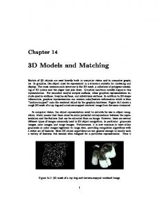
5. Experiments Synthetic data. We sample synthetic data to have ground truth information for comparison. We sample from linear DCCA which extends linear CCA (7) such that each view is xj ∼ Poisson(Dj α + Fj βj ). The sources α ∼ Gamma(c, b) and the noise sources βj ∼ Gamma(cj , bj ), for j = 1, 2, are sampled from the gamma distribution (where b is the rate parameter). Let sj ∼ Poisson(Dj α) be the part of the sample due to the sources and nj ∼ Poisson(Fj βj ) be the part of the sample due to the noise (i.e., xj = sj + nj ). Then we define the expected sample length noise, respectively, as Ljs := P due to the sources andP E[ m sjm ] and Ljn := E[ m njm ]. For sampling, the target values Ls = L1s = L2s and Ln = L1n = L2n are fixed and the parameters b and bj are accordingly set to ensure these values: b = Kc/Ls and bj = Kj cj /Ln (see Appendix B.2 of Podosinnikova et al. (2015)). For the larger dimensional example (Fig. 2, right), each column of the matrices Dj and Fj , for j = 1, 2, is sampled from the symmetric Dirichlet distribution with the concentration parameter equal to 0.5. For the smaller 2D example (Fig. 2, left), they are fixed: D1 = D2 with [D1 ]1 = [D1 ]2 = 0.5 and F1 = F2 with [F1 ]11 = [F1 ]22 = 0.9 and [F1 ]12 = [F1 ]21 = 0.1. For each experiment, Dj and Fj , for j = 1, 2, are sampled once and, then, the x-

Beyond CCA: Moment Matching for Multi-View Models 0.5

0.5

ℓ1 -error

0.4 0.3

1000 X1 D1 F11 F12

800 600

0.2

NMF NMF° DICA DCCA DCCAg

0.4

ℓ1 -error

NMF NMF° DICA DCCA DCCAg

0.3 0.2

400

0.1 0

0.1

200

0

2000

4000

6000

8000

Number of samples

10000

0

0 0

200

400

600

800

1000

0

2000

4000

6000

8000

10000

Number of samples

Figure 2. Synthetic experiment with discrete data. Left (2D example): M1 = M2 = K1 = K2 = 2, K = 1, c = c1 = c2 = 0.1, and Ls = Ln = 100; middle (2D data): the x1 -observations and factor loading matrices for the 2D example (F1j denotes the j-th column of the noise factor matrix F1 ); right (20D example): M1 = M2 = K1 = K2 = 20, K = 10, Ls = Ln = 1, 000, c = 0.3, and c1 = c2 = 0.1. nato otan work travail board commission nisga nisga kosovo kosovo workers négociations wheat blé treaty autochtones strike travailleurs farmers agriculteurs aboriginal traité forces militaires military guerre legislation grève grain administration agreement accord union emploi producers producteurs right droit war international troops pays agreement droit amendment grain land nations country réfugiés labour syndicat market conseil reserve britannique world situation right services directors ouest national indiennes national paix services accord western amendement british terre peace yougoslavie negotiations voix election comité columbia colombie Table 1. Factor loadings (a.k.a. topics) extracted from the Hansard collection for K = 20 with DCCA.

observations are sampled for different sample sizes N = {500, 1, 000, 2, 000, 5, 000, 10, 000}, 5 times for each N . Metric. The evaluation is performed on a matrix D obtained by stacking D1 and D2 vertically (see also the comment after Thm. 1). As in Podosinnikova et al. (2015), we use as evaluation metric the normalized `1 b and the true matrix error between a recovered matrix D b D) := D with the best permutation of columns err1 (D, P b 1 minπ∈PERM 2K k kdπk − dk k1 ∈ [0, 1]. The minimization is over the possible permutations π ∈ PERM of the b and can be efficiently obtained with the Huncolumns of D garian algorithm for bipartite matching. The (normalized) `1 -error takes the values in [0, 1] and smaller values of this error indicate better performance of an algorithm. Algorithms. We compare DCCA (implementation with the S- and T-cumulants) and DCCAg (implementation with the generalized S-covariance matrices and the processing points initialized as described in Appendix E.4) to DICA and the non-negative matrix factorization (NMF) algorithm with multiplicative updates for divergence (Lee & Seung, 2000). To run DICA or NMF, we use the stacking trick (8). DCCA is set to estimate K components. DICA is set to estimate either K0 = K+K1 +K2 or M = M1 +M2 components (whichever is the smallest, since DICA cannot work in the over-complete case). NMF is always set to estimate K0 components. For the evaluation of DICA/NMF, the K columns with the smallest `1 -error are chosen. NMF◦ stands for NMF initialized with a matrix D of the form (8) with induced zeros; otherwise NMF is initialized with (uniformly) random non-negative matrices. The running times

are discussed in Appendix G.5. Synthetic experiment. We first perform an experiment with discrete synthetic data in 2D (Fig. 2) and then repeat the same experiment when the size of the problem is 10 times larger. In practice, we observed that for K0 < M all models work approximately equally well, except for NMF which breaks down in high dimensions. In the overcomplete case as in Fig. 2, DCCA works better. A continuous analogue of this experiment is presented in Appendix G.1. Real data (translation). Following Vinokourov et al. (2002), we illustrate the performance of DCCA by extracting bilingual topics from the Hansard collection (Vinokourov & Girolami, 2002) with aligned English and French proceedings of the 36-th Canadian Parliament. In Table 1, we present some of the topics extracted after running DCCA with K = 20 (see all the details in Appendices G.3 and G.4). The (Matlab/C++) code for reproducing the experiments of this paper is available at https://github.com/anastasia-podosinnikova/cca. Conclusion We have proposed the first identifiable versions of CCA, together with moment matching algorithms which allow the identification of the loading matrices in a semi-parametric framework, where no assumptions are made regarding the distribution of the source or the noise. We also introduce new sets of moments (our generalized covariance matrices), which could prove useful in other settings.


Acknowledgements This work was partially supported by the MSR-Inria Joint Center.

Browne, M.W. The maximum-likelihood solution in interbattery factor analysis. Br. J. Math. Stat. Psychol., 32(1): 75–86, 1979.

References

Bunse-Gerstner, A., Byers, R., and Mehrmann, V. Numerical methods for simultaneous diagonalization. SIAM J. Matrix Anal. Appl., 14(4):927–949, 1993.

Anandkumar, A. and Sedghi, H. Learning mixed membership community models in social tagging networks through tensor methods. CoRR, arXiv:1503.04567v2, 2015.

Cardoso, J.-F. Source separation using higher order moments. In Proc. ICASSP, 1989.

Anandkumar, A., Foster, D.P., Hsu, D., Kakade, S.M., and Liu, Y.-K. A spectral algorithm for latent Dirichlet allocation. In Adv. NIPS, 2012. Anandkumar, A., Foster, D.P., Hsu, D., Kakade, S.M., and Liu, Y.-K. A spectral algorithm for latent Dirichlet allocation. CoRR, abs:1204.6703v4, 2013. Anandkumar, A., Ge, R., Hsu, D., Kakade, S.M., and Telgarsky, M. Tensor decompositions for learning latent variable models. J. Mach. Learn. Res., 15:2773–2832, 2014. Arora, S. and Kannan, R. Learning mixtures of separated nonspherical Gaussians. Ann. Appl. Probab., 15(1A): 69–92, 2005. Arora, S., Ge, R., and Moitra, A. Learning topic models – Going beyond SVD. In Proc. FOCS, 2012.

Cardoso, J.-F. and Comon, P. Independent component analysis, A survey of some algebraic methods. In Proc. ISCAS, 1996. Cardoso, J.-F. and Souloumiac, A. Blind beamforming for non Gaussian signals. In IEE Proc-F, 1993. Cardoso, J.-F. and Souloumiac, A. Jacobi angles for simultaneous diagonalization. SIAM J. Mat. Anal. Appl., 17 (1):161–164, 1996. Comon, P. Independent component analysis, A new concept? Signal Process., 36(3):287–314, 1994. Comon, P. and Jutten, C. Handbook of Blind Source Separation: Independent Component Analysis and Applications. Academic Press, 2010. Eberlein, P.J. A Jacobi-like method for the automatic computation of eigenvalues and eigenvectors of an arbitrary matrix. J. Soc. Indust. Appl. Math., 10(1):74–88, 1962. Fu, T. and Gao, X. Simultaneous diagonalization with similarity transformation for non-defective matrices. In Proc. ICASSP, 2006.

Arora, S., Ge, R., Halpern, Y., Mimno, D., Moitra, A., Sontag, D., Wu, Y., and Zhu, M. A practical algorithm for topic modeling with provable guarantees. In Proc. ICML, 2013.

Ge, R. and Zou, J. Rich component analysis. In Proc. ICML, 2016.

Bach, F. and Jordan, M.I. Kernel independent component analysis. J. Mach. Learn. Res., 3:1–48, 2003.

Golub, G.H. and Van Loan, C.F. Matrix Computations. John Hopkins University Press, 3rd edition, 1996.

Bach, F. and Jordan, M.I. A probabilistic interpretation of canonical correlation analysis. Technical Report 688, Department of Statistics, University of California, Berkeley, 2005.

Gong, Y., Ke, Q., Isard, M., and Lazebnik, S. A multi-view embedding space for modeling internet images, tags, and their semantics. Int. J. Comput. Vis., 106(2):210–233, 2014.

Balle, B., Hamilton, W.L., and Pineau, J. Method of moments for learning stochastic languages: Unified presentation and empirical comparison. In Proc. ICML, 2014. Bartholomew, D.J. Latent Variable Models and Factor Analysis. Wiley, 1987. Basilevsky, A. Statistical Factor Analysis and Related Methods: Theory and Applications. Wiley, 1994. Blei, D.M., Ng, A.Y., and Jordan, M.I. Latent Dirichlet allocation. J. Mach. Learn. Res., 3:993–1022, 2003.

Haghighi, A., Liang, P., Kirkpatrick, T.B., and Klein, D. Learning bilingual lexicons from monolingual corpora. In Proc. ACL, 2008. Halko, N., Martinsson, P.G., and Tropp, J.A. Finding structure with randomness: Probabilistic algorithms for constructing approximate matrix decompositions. SIAM Rev., 53(2):217–288, 2011. Hardoon, D.R., Szedmak, S.R., and Shawe-Taylor, J.R. Canonical correlation analysis: An overview with application to learning methods. Neural Comput., 16(12): 2639–2664, 2004.


Hotelling, H. Relations between two sets of variates. Biometrica, 28(3/4):321–377, 1936.

Shawe-Taylor, J.R. and Cristianini, N. Kernel Methods for Pattern Analysis. Cambridge University Press, 2004.

Hsu, D. and Kakade, S.M. Learning mixtures of spherical Gaussians: Moment methods and spectral decompositions. In Proc. ITCS, 2013.

Slapak, A. and Yeredor, A. Charrelation matrix based ICA. In Proc. LVA ICA, 2012a.

Iferroudjene, R., Abed Meraim, K., and Belouchrani, A. A new Jacobi-like method for joint diagonalization of arbitrary non-defective matrices. Appl. Math. Comput., 211:363–373, 2009. Janzamin, M., Sedghi, H., and Anandkumar, A. Beating the perils of non-convexity: Guaranteed training of neural networks using tensor methods. CoRR, arXiv:1506.08473v3, 2016. Jutten, C. Calcul neuromimétique et traitement du signal: Analyse en composantes indépendantes. PhD thesis, INP-USM Grenoble, 1987.

Slapak, A. and Yeredor, A. Charrelation and charm: Generic statistics incorporating higher-order information. IEEE Trans. Signal Process., 60(10):5089–5106, 2012b. Socher, R. and Fei-Fei, L. Connecting modalities: Semisupervised segmentation and annotation of images using unaligned text corpora. In Proc. CVPR, 2010. Song, L., Anandkumar, A., Dai, B., and Xie, B. Nonparametric estimation of multi-view latent variable models. In Proc. ICML, 2014. Stewart, G.W. and Sun, J. Matrix Perturbation Theory. Academic Press, 1990.

Jutten, C. and Hérault, J. Blind separation of sources, part I: An adaptive algorithm based on neuromimetric architecture. Signal Process., 24(1):1–10, 1991.

Sübakan, Y.C., Traa, J., and Smaragdis, P. Spectral learning of mixture of hidden Markov models. In Adv. NIPS, 2014.

Klami, A., Virtanen, S., and Kaski, S. Bayesian exponential family projections for coupled data sources. In Proc. UAI, 2010.

Tipping, M.E. and Bishop, C.M. Probabilistic principal component analysis. J. R. Stat. Soc. Series B, 61(3):611– 622, 1999.

Klami, A., Virtanen, S., and Kaski, S. Bayesian canonical correlation analysis. J. Mach. Learn. Res., 14:965–1003, 2013.

Todros, K. and Hero, A.O. Measure transformed independent component analysis. CoRR, arXiv:1302.0730v2, 2013.

Kolda, T.G. and Bader, B.W. Tensor decompositions and applications. SIAM Rev., 51(3):455–500, 2009.

Tung, H.-Y. and Smola, A. Spectral methods for Indian buffet process inference. In Adv. NIPS, 2014.

Kuleshov, V., Chaganty, A.T., and Liang, P. Tensor factorization via matrix factorization. In Proc. AISTATS, 2015.

Vinokourov, A. and Girolami, M. A probabilistic framework for the hierarchic organisation and classification of document collections. J. Intell. Inf. Syst., 18(2/3):153– 172, 2002.

Lee, D.D. and Seung, H.S. Algorithms for non-negative matrix factorization. In Adv. NIPS, 2000. Luciani, X. and Albera, L. Joint eigenvalue decomposition using polar matrix factorization. In Proc. LVA ICA, 2010.

Vinokourov, A., Shawe-Taylor, J.R., and Cristianini, N. Inferring a semantic representation of text via crosslanguage correlation analysis. In Adv. NIPS, 2002.

Murphy, K.P. Machine Learning: A Probabilistic Perspective. MIT Press, 2012.

Virtanen, S. Bayesian exponential family projections. Master’s thesis, Aalto University, 2010.

Podosinnikova, A., Bach, F., and Lacoste-Julien, S. Rethinking LDA: Moment matching for discrete ICA. In Adv. NIPS, 2015.

Wang, Y. and Zhu, J. Spectral methods for supervised topic models. In Adv. NIPS, 2014.

Roweis, S. EM algorithms for PCA and SPCA. In Adv. NIPS, 1998. Ruhe, A. On the quadratic convergene of a generalization of the Jacobi method to arbitrary matrices. BIT Numer. Math., 8(3):210–231, 1968.

Yeredor, A. Blind source separation via the second characteristic function. Signal Process., 80(5):897–902, 2000.


6. Appendix

A.2. NAMING CONVENTION

The appendix is organized as follows.

A number of models have the linear form x = Dα. Depending on the context, the matrix D is called differently: topic matrix3 in the topic learning context, factor loading or projection matrix in the FA and/or PPCA context, mixing matrix in the ICA context, or dictionary in the dictionary learning context.

- In Appendix A, we summarize our notation. - In Appendix B, we present the proof of Theorem 1 stating the identifiability of the CCA models (4)–(6). - In Appendix C, we provide some details for the generalized covariance matrices: the form of the generalized covariance matrices of independent variables (Appendix C.1), the derivations of the diagonal form of the generalized covariance matrices of discrete ICA (Appendix C.3), the derivations of the diagonal form of the generalized covariance matrices of the CCA models (4)–(6) (Appendix C.4), and approximation of the T-cumulants with the generalized covariance matrix (Appendix C.5). - In Appendix D, we provide expressions for natural finite sample estimators of the generalized covariance matrices and the T-cumulant tensors for the considered CCA models. - In Appendix E, we discuss some rather technical implementation details: computation of whitening matrices (Appendix E.2), selection of the projection vectors for the T-cumulants and the processing points for the generalized covariance matrices (Appendix E.4), and the final estimation of the factor loading matrices (Appendix E.5). - In Appendix F, we describe the non-orthogonal joint diagonalization algorithms used in this paper. - In Appendix G, we present some supplementary experiments: a continuous analog of the synthetic experiment from Section 5 (Appendix G.1), an experiment to analyze the sensitivity of the DCCA algorithm with the generalized S-covariance matrices to the choice of the processing points (Appendix G.2), and a detailed description of the experiment with the real data from Section 5 (Appendices G.3 and G.4).

Our linear multi-view models, x1 = D1 α and x2 = D2 α, are closely related the linear models mentioned above. For example, due to the close relation of DCCA and DICA, the former is closely related to the multi-view topic models (see, e.g., Blei & Jordan, 2003). In this paper, we refer to D1 and D2 as the factor loading matrices, although depending on contex any other name can be used. B. Identifiability In this section, we prove that the factor loading matrices D1 and D2 of the non-Gaussian CCA (4), discrete CCA (5), and mixed CCA (6) models are identifiable up to permutation and scaling if at most one source αk is Gaussian. We provide a complete proof for the non-Gaussian CCA case and show that the other two cases can be proved by analogy. B.1. I DENTIFIABILITY OF NON -G AUSSIAN CCA (4) The proof uses the notion of the second characteristic function (SCF) of a random variable x ∈ RM : >

φx (t) = log E(eit

),

for all t ∈ RM . The SCF completely defines the probability distribution of x (see, e.g., Jacod & Protter, 2004). Important difference between the SCF and the cumulant generating function (19) is that the former always exists. The following property of the SCF is of central importance for the proof: if two random variables, z1 and z2 , are in> dependent, then φA1 z1 +A2 z2 (t) = φz1 (A> 1 t) + φz2 (A2 t), where A1 and A2 are any matrices of compatible sizes. We can now use our CCA model to derive an expression of φx (t). Indeed, defining a vector x by stacking the vectors x1 and x2 , the SCF of x for any t = [t1 ; t2 ], takes the form >

>

φx (t) = log E(eit1 x1 +it2 x2 )

A. Notation A.1. N OTATION SUMMARY The vector α ∈ RK refers to the latent sources. Unless otherwise specified, the components α1 , . . . , αK of the vector α are mutually independent. For a linear single-view model, x = Dα, the vector x ∈ RM denotes the observation vector (sensors or documents), where M is, respectively, the number of sensors or the vocabulary size. For the two-view model, x, M , and D take the indices 1 and 2.

x

(a)

= log E(eiα

>

> (D1> t1 +D2> t2 )+iε> 1 t1 +iε2 t2

(b)

>

(D1> t1 +D2> t2 )

= log E(eiα

+ log E(e

)

)

iε> 1 t1

>

) + log E(eiε2 t2 )

= φα (D1> t1 + D2> t2 ) + φε1 (t1 ) + φε2 (t2 ), 3

Note that Podosinnikova et al. (2015) show that DICA is closely connected (and under some conditions is equivalent) to latent Dirichlet allocation (Blei et al., 2003).


where in (a) we substituted the definition (4) of x1 and x2 and in (b) we used the independence α ⊥ ⊥ ε1 ⊥ ⊥ ε2 . Therefore, the blockwise mixed derivatives of φx are equal to ∂1 ∂2 φx (t) =

D1 φ00α (D1> t1

+

D2> t2 )D2> ,

For simplicity, we first prove the identifiability result when all components of the common sources are non-Gaussian. The high level idea of the proof is as follows. We assume two different representations of x1 and x2 and using (32) and the independence of the components of α and the noises, we first show that the two potential dictionaries are related by an orthogonal matrix (and not any invertible matrix), and then show that this implies that the two potential sets of independent components are (orthogonal) linear combinations of each other, which, for non-Gaussian components which are not reduced to point masses, imposes that this orthogonal transformation is the combination of a permutation matrix and marginal scaling—a standard result from the ICA literature (Comon, 1994, Theorem 11). Let us then assume that two equivalent representations of non-Gaussian CCA exist:

x2 = D2 α + ε2 = E2 β + η2 ,

(33)

where the other sources β = (β1 , . . . , βK ) are also assumed mutually independent and non-degenerate. As a standard practice in the ICA literature and without loss of generality as the sources have non-degenerate components, one can assume that the sources have unit variances, i.e. cov(α, α) = I and cov(β, β) = I, by respectively rescaling the columns of the factor loading matrices. Under this assumption, the two expressions of the cross-covariance matrix are cov(x1 , x2 ) = D1 D2> = E1 E2> ,

(34)

which, given that D1 , D2 have full rank, implies that4 E1 = D1 Q,

E2 = D2 Q−> ,

φ00α (D1> t1 + D2> t2 )

(32)

where ∂1 ∂2 φx (t) := ∇t1 ∇t2 φx (h(t1 , t2 )) ∈ RM1 ×M2 and φ00α (u) := ∇2u φα (u), does not depend on the noise vectors ε1 and ε2 .

x1 = D1 α + ε1 = E1 β + η1 ,

for all t1 ∈ RM1 and t2 ∈ RM2 . Since the matrices D1 and D2 have full rank, this can be rewritten as

(35)

where Q ∈ RK×K is some invertible matrix. Substituting the representations (33) into the blockwise mixed derivatives of the SCF (32) and using the expressions (35) give D1 φ00α (D1> t1 + D2> t2 )D2>

= Qφ00β (Q> D1> t1 + Q−1 D2> t2 )Q−1 , which holds for all t1 ∈ RM1 and t2 ∈ RM2 . Moreover, still since D1 and D2 have full rank, we have, for any u1 , u2 ∈ RK the existence of t1 ∈ RM1 and t2 ∈ RM2 , such that u1 = D1> t1 and u2 = D2> t2 , that is, φ00α (u1 + u2 ) = Qφ00β (Q> u1 + Q−1 u2 )Q−1 , for all u1 , u2 ∈ RK . We will now prove two facts: (F1) For any vector v ∈ RK , then φ00β ((Q> Q − I)v) = −I, which will imply that QQ> = I because of the nonGaussian assumptions. (F2) If QQ> = I, then φ00α (u) = φ00Qβ (u) for any u ∈ RK , which will imply that Q is the composition of a permutation and a scaling. This will end the proof. Proof of fact (F1). By letting u1 = Qv and u2 = −Qv, we get: φ00α (0) = Qφ00β ((Q> Q − I)v)Q−1 , (37) Since5 φ00α (0) = −cov(α) = −I, one gets φ00β ((Q> Q − I)v) = −I, for any v ∈ RK . Using the property that φ00A> β (v) = A> φ00β (Av)A for any matrix A, and in particular with A = Q> Q − I, we have that φ00A> β (v) = −A> A, i.e. is constant. If the second derivative of a function is constant, the function is quadratic. Therefore, φA> β (·) is a quadratic function. Since the SCF completely defines the distribution of its variable (see,e.g., Jacod & Protter (2004)), A> β must be Gaussian (the SCF of a Gaussian random variable is a quadratic function). Given Lemma 9 from Comon (1994) (i.e., Cramer’s lemma: a linear combination of nonGaussian random variables cannot be Gaussian unless the coefficients are all zero), this implies that A = 0, and hence Q> Q = I, i.e., Q is an orthogonal matrix. Proof of fact (F2). Plugging Q> = Q−1 into (36), with u1 = 0 and u2 = u, gives φ00α (u) = Qφ00β (Q> u)Q> = φ00Qβ (u),

= D1 Qφ00β (Q> D1> t1 + Q−1 D2> t2 )Q−1 D2> , 4

The fact that D1 , D2 have full rank and that E1 , E2 have K columns, combined with (34), implies that E1 , E2 have also full rank.

(36)

5

> iu> α

Note that ∇2u φα (u) = − E(αα iue> α E(e

where Eα (u) =

> E(αeiu α ) > E(eiu α )

.

)

)

(38)

+ Eα (u)Eα (u)> ,


for any u ∈ RK . By integrating both sides of (38) and using φα (0) = φQβ (0) = 0, we get that φα (u) = φQβ (u) + iγ > u for all u ∈ RK for some constant vector γ. Using again that the SCF completely defines the distribution, it follows that α − γ and Qβ have the same distribution. Since both α and β have independent components, this is only possible when Q = ΛP , where P is a permutation matrix and Λ is some diagonal matrix (Comon, 1994, Theorem 11). B.2. C ASE OF A SINGLE G AUSSIAN SOURCE Without loss of generality, we assume that the potential Gaussian source is the first one for α and β. The first change is in the proof of fact (F1). We use the same argument up to the point where we conclude that A> β is a Gaussian vector. As only β1 can be Gaussian, Cramer’s lemma implies that only the first row of A can have nonzero components, that is A = Q> Q − I = e1 f > , where e1 is the first basis vector and f any vector. Since Q> Q is symmetric, we must have Q> Q = I + ae1 e> 1, where a is a constant scalar different than −1 as Q> Q is invertible. This implies that Q> Q is an invertible diagonal matrix Λ, and hence QΛ−1/2 is an orthogonal matrix, which in turn implies that Q−1 = Λ−1 Q> . Plugging this into (36) gives, for any u1 and u2 : φ00α (u1 + u2 ) = Qφ00β (Q> u1 + Λ−1 Q> u2 )Λ−1 Q> .

B.3. I DENTIFIABILITY OF DISCRETE CCA (5) AND MIXED CCA (6) Given the discrete CCA model, the SCF φx (t) takes the form φx (t) = φα (D1> (eit1 − 1) + D2> (eit2 − 1)) + φε1 (eit1 − 1) + φε2 (eit2 − 1), where eitj , for j = 1, 2, denotes a vector with the m-th element equal to ei[tj ]m , and we used the arguments analogous with the non-Gaussian case. The rest of the proof extends with a correction that sometimes one has to replace Dj with diag[eitj ]Dj and that uj = Dj> (eitj − 1) for j = 1, 2. For the mixed CCA case, only the part related to x2 and D2 changes in the same way as for the discrete CCA case. C. The generalized expectation and covariance matrix C.1. T HE GENERALIZED EXPECTATION AND COVARIANCE MATRIX OF THE SOURCES

Note that some properties of the generalized expectation and covariance matrix, defined in (20) and (21), and their natural finite sample estimators are analyzed by Slapak & Yeredor (2012b). Note also that we find the name “generalized covariance matrix” to be more meaningful than “charrelation” matrix as was proposed by previous authors (see, e.g. Slapak & Yeredor, 2012a;b). The sources α = (α1 , . . . , αK ) are mutually independent. Therefore, for some h ∈ RK , their CGF (19) Kα (h) = > log E(eα h ) takes the form X Kα (h) = log E(eαk hk ) . k

φ00β

Given that diagonal matrices commute and that is diagonal for independent sources (see Appendix C.1), this leads to

Therefore, the k-th element of the generalized expectation (20) of α is (separable in αk ) [Eα (h)]k =

φ00α (u1 +u2 )

=

QΛ−1/2 φ00β (Q> u1 +Λ−1 Q> u2 )Λ−1/2 Q> .

For any given v ∈ RK , we are looking for u1 and u2 such that Q> u1 + Λ−1 Q> u2 = Λ−1/2 Q> v and u1 + u2 = v, which is always possible by setting Q> u2 = (Λ−1/2 + I)−1 Q> v and Q> u1 = Q> v − Q> u2 by using the special structure of Λ. Thus, for any v,

E(αk eαk hk ) E(eαk hk )

(39)

and the generalized covariance (21) of α is diagonal due to the separability and its k-th diagonal element is [Cα (h)]kk =

E(αk2 eαk hk ) 2 − [Eα (h)]k . E(eαk hk )

(40)

C.2. S OME EXPECTATIONS OF A P OISSON RANDOM VARIABLE

φ00α (v)

=

QΛ−1/2 φ00β (Λ−1/2 Q> v)Λ−1/2 Q>

=

φ00QΛ−1/2 β (v).

Integrating as previously, this implies that the characteristic function of α and QΛ−1/2 β differ only by a linear function iγ > v, and thus, that α − γ and QΛ−1/2 β have the same distribution. This in turn, from Comon (1994, Theorem 11), implies that QΛ−1/2 is a product of a scaling and a permutation, which ends the proof.

Let x ∈ RM be a multivariate Poisson random variable M with mean y ∈ RM + . Then, for some t ∈ R , E(et

>

x

E(xm et

>

x

E(xm xm0 et

>

x

) = ey

>

(et −1)

,

>

t

) = ym etm ey (e −1) , > > t E(x2m et x ) = ym etm + 1 ym etm ey (e −1) , ) = ym etm ym0 etm0 ey

>

(et −1)

,

m 6= m0 ,


where et denotes an M -vector with the m-th element equal to etm . C.3. T HE GENERALIZED EXPECTATION AND COVARIANCE MATRIX OF DISCRETE ICA In this section, we use the expectations of a Poisson random variable presented in Appendix C.2. Given the discrete ICA model (9), the generalized expectation (20) of x ∈ RM takes the form h i t> x E E(xe |α) E(xe ) = Ex (t) = E(et> x ) E E(et> x |α) t> x

>

E(αeα h(t) ) = diag[e ]D E(eα> h(t) ) = diag[et ]DEα (h(t)), t

where t ∈ RM is a parameter, h(t) = D> (et − 1), and et denotes an M -vector with the m-th element equal to etm . Note that in the last equation we used the definition (20) of the generalized expectation Eα (·). Further, the generalized covariance (21) of x takes the form >

E(xx> et x ) − Ex (t)Ex (t)> E(et> x ) h i > E E(xx> et x |α) − Ex (t)Ex (t)> . = E E(et> x |α)

Cx (t) =

Plugging into this expression the expression for Ex (t) and E(xx> et

>

x

>

|α) = diag[et ]DE(αα> eα h(t) )D> diag[et ] h i > + diag[et ]diag DE(αeα h(t) )

written as >

>

Kx (t) = log E(et1 x1 +t2 x2 ) i h > > = log E E(et1 x1 +t2 x2 | α, ε1 , ε2 ) i h > > (a) = log E E(et1 x1 | α, ε1 )E(et2 x2 | α, ε2 ) > > t2 (b) = log E et1 (D1 α+ε1 ) e(D2 α+ε2 ) (e −1) > t > > (c) 2 = log E eα h(t) + log E eε2 (e −1) + log E(et1 ε1 ), where h(t) = (D1> t1 + D2> (et2 − 1), in (a) we used the conditional independence of x1 and x2 , in (b) we used the first expression from Appendix C.2, and in (c) we used the independence assumption (3). The generalized CCA S-covariance matrix is defined as S12 (t) := ∇t2 ∇t1 Kx (t). Its gradient with respect to t1 is >

∇t1 Kx (t) =

where the last term does not depend on t2 . Computing the gradient of this expression with respect to t2 gives > S12 (t) = D1 Cα (h(t)) diag[et2 ]D2 , where we substituted expression (40) for the generalized covariance of the independent sources. C.5. A PPROXIMATION OF THE T- CUMULANTS WITH THE GENERALIZED COVARIANCE MATRIX

Let fmm0 (t) = [Cx (t)]mm0 be a function R → RM corresponding to the (m, m0 )-th element of the generalized covariance matrix. Then the following holds for its directional derivative at t0 along the direction t: h∇fmm0 (t0 ), ti = lim

δ→0

we get Cx (t) = diag[Ex (t)] + diag[et ]DCα (h(t))D> diag[et ], where we used the definition (21) of the generalized covariance of α. C.4. T HE GENERALIZED CCA S- COVARIANCE MATRIX In this section we sketch the derivation of the diagonal form (27) of the generalized S-covariance matrix of mixed CCA (6). Expressions (25) and (26) can be obtained in a similar way. Denoting x = [x1 ; x2 ] and t = [t1 ; t2 ] (i.e. stacking the vectors as in (8)), the CGF (19) of mixed CCA (6) can be

>

D1 E(αeα h(t) ) E(ε1 et1 ε1 ) , + > E(eα> h(t) ) E(et1 ε1 )

fmm0 (t0 + δt) − fmm0 (t0 ) , δ

where h·, ·i stands for the inner product. Therefore, when using the fact that ∇f (t0 ) = ∇Cx (t) is the generalized cumulant of x at t0 and the definition of a projection of a tensor onto a vector (42), one obtains for t0 = 0 the approximation of the cumulant cum(x) with the generalized covariance matrix Cx (t). Let us define v1 = W1> u1 and v1 = W2> u2 for some u1 , u2 ∈ RK . Then, approximations for the Tcumulants (17) of discrete CCA take the following form: W1 T121 (v1 )W2 is approximated by the generalized Scovariances (24) S12 (t) via the following expression W1 S12 (δt1 )W2> − W1 S12 (0)W2> δ − W1 diag(v1 )S12 W2> ,

W1 T121 (v1 )W2 ≈


v1 where t1 = and W1 T122 (v2 )W2 is approximated by 0 the generalized S-covariances S12 (t) via W1 S12 (δt2 )W2> − W1 S12 (0)W2> δ − W1 S12 diag(v2 )W2> ,

W1 T122 (v2 )W2 ≈

where t2 =

0 and δ are chosen to be small. v2

D. Finite sample estimators D.1. F INITE SAMPLE ESTIMATORS OF THE GENERALIZED EXPECTATION AND COVARIANCE MATRIX

Following Yeredor (2000); Slapak & Yeredor (2012b), we use the most direct way of defining the finite sample estimators of the generalized expectation (20) and covariance matrix (21). Given a finite sample X = {x1 , x2 , . . . , xN }, an estimator of the generalized expectation is P n xn wn Ebx (t) = P n wn

cum(x1 , x2 ), takes the form h i b 1 )E(x b 2 )> , Sb12 = η1 X1 X2> − N E(x b 1 ) = N −1 where E(x and η1 = 1/(N − 1).

P

(41)

b 2 ) = N −1 P n x2n , x1n , E(x

n

Substitution of the finite sample estimators of the 2nd and 3rd cumulants (see, e.g., Appendix C.4 of Podosinnikova et al. (2015)) into the definition of the DCCA Tcumulants (17) leads to the following expressions c1 Tb12j (vj )W c > = η2 [(W c1 X1 )diag(X > vj )] ⊗ (W c2 X2 ) W 2 j b j )i2N [W b 1 )] ⊗ [W b 2 )] c1 E(x c2 E(x + η2 hvj , E(x b j )i(W c1 X1 ) ⊗ (W c2 X2 ) − η2 hvj , E(x b 2 )] c1 X1 )(Xj> vj )] ⊗ [W c2 E(x − η2 [(W b 1 )] ⊗ [(W c1 E(x c2 X2 )(Xj> vj )] − η2 [W (j)

(j)

c X1 ) ⊗ (W c X2 ) − η1 (W 1 2 b 1 )] ⊗ [W b 2 )], c (j) E(x c (j) E(x + η1 N [W 1 2 c (1) = W c1 diag(v1 ), where η2 = N/((N −1)(N −2)) and W 1 (1) (2) (2) c c c c c c W2 = W2 , W1 = W1 , and W2 = W2 diag(v2 ).

>

where weights wn = et xn and an estimator of the generalized covariance is P > n xn xn w n b P Cx (t) = − Ebx (t)Ebx (t)> . n wn

c1 and W c2 denote whitening maIn the expressions above, W c1 Sb12 W c > = I. trices of Sb12 , i.e. such that W 2 E. Implementation details E.1. C ONSTRUCTION OF S- AND T- CUMULANTS

Similarly, an estimator of the generalized S-covariance matrix is then P P > P > n x1n wn n x2n wn n x1n x2n wn b P P − P , Cx1 ,x2 (t) = n wn n wn n wn

By analogy with Podosinnikova et al. (2015), the target matrices for joint diagonalization can be constructed from Sand T-cumulants.

where x = [x1 ; x2 ] and t = [t1 ; t2 ] for some t1 ∈ RM1 and t2 ∈ RM2 .

When dealing with the S- and T-cumulants, the target matrices are obtained via tensor projections. We define a projection T (v) ∈ RM1 ×M2 of a third-order tensor T ∈ RM1 ×M2 ×M3 onto a vector v ∈ RM3 as

Some properties of these estimators are analyzed by Slapak & Yeredor (2012b). D.2. F INITE SAMPLE ESTIMATORS OF THE DCCA

[T (v)]m1 m2 :=

M3 X

[T ]m1 m2 m3 vm3 .

(42)

m3 =1

CUMULANTS

In this section, we sketch the derivation of unbiased finite sample estimators for the CCA cumulants S12 , T121 , and T122 . Since the derivation is nearly identical to the derivation of the estimators for the DICA cumulants (see Appendix F.2 of Podosinnikova et al. (2015)), all details are omitted. Given a finite sample X1 = {x11 , x12 , . . . , x1N } and X2 = {x21 , x22 , . . . , x2N }, the finite sample estimator of the discrete CCA S-covariance (15), i.e., S12 :=

Note that the projection T (v) is a matrix. Therefore, given 2P vectors {v11 , v21 , v12 , v22 , . . . , v1P , v2P }, one can construct 2P + 1 matrices {S12 , T121 (v1p ), T122 (v2p ), for p = 1, . . . , P }, (43) which have the diagonal form (16) and (18). Importantly, the tensors are never constructed (see Anandkumar et al. (2012; 2014); Podosinnikova et al. (2015) and Appendix D.2).


E.2. C OMPUTATION OF WHITENING MATRICES One can compute such whitening matrices (29) via the singular value decomposition (SVD) of S12 . Let S12 = U ΣV > be the SVD of S12 , then one can define W1 = U1:K Λ and W2 = V1:K Λ, where U1:K and V1:K are the first K left- and right-singular vectors and Λ = −1/2 −1/2 diag(σ1 , . . . , σK ) and σ1 , . . . , σK are the K largest singular values. Although SVD is computed only once, the size of the matrix S12 can be significant even for storage. To avoid construction of this large matrix and speed up SVD, one can use randomized SVD techniques (Halko et al., 2011). Indeed, since the sample estimator Sb12 has the form (41), one can reduce this matrix by sampling two Gaussian random ˜ ˜ ˜ is matrices Ω1 ∈ RK×M1 and Ω2 ∈ RK×M2 , where K slightly larger than K. Now, if U and V are the K largest singular vectors of the reduced matrix Ω1 Sb12 Ω2 , then Ω†1 U and Ω†2 V are approximately (and up to permutation and scaling of the columns) the K largest singular vectors of Sb12 . E.3. A PPLYING WHITENING TRANSFORM TO DCCA T- CUMULANTS Transformation of the T-cumulants (43) with whitening matrices W1 and W2 gives new tensors Tb12j ∈ RK×K×K : Tb12j := T12j ×1 W1> ×2 W2> ×3 Wj> ,

(44)

where j = 1, 2. Combining this transformation with the projection (42), one obtains 2P + 1 matrices W1 S12 W2> , W1 T12j (Wj> ujp )W2> ,

(45)

where p = 1, . . . , P and j = 1, 2 and we used vjp = Wj> ujp to take into account whitening along the third direction. By choosing ujp ∈ RK to be the canonical vectors of the RK , the number of tensor projections is reduced from M = M1 + M2 to 2K. E.4. C HOICE OF PROJECTION VECTORS OR PROCESSING POINTS

For the T-cumulants (43), we choose the K projection vectors as v1p = W1> ep and v2p = W2> ep , where ep is one of the columns of the K-identity matrix (i.e., a canonical vector). For the generalized S-covariances (28), we choose the processing points as t1p = δ1 v1p and t2p = δ2 v2p , where δj , P for j = 1, 2 are set to a small value such as 0.1 divided by m E(|xjm |)/Mj , for j = 1, 2. When projecting a tensor T12j onto a vector, part of the information contained in this tensor gets lost. To preserve all information, one could project a tensor T12j onto the canonical basis of RMj to obtain Mj matrices. However, this would be an expensive operation in terms of both

memory and computational time. In practice, we use the fact, that the tensor T12j , for J = 1, 2, is transformed with whitening matrices (44). Hence, the projection vector has to include multiplication by the whitening matrices. Since they reduce the dimension to K, choosing the canonical basis in RK becomes sufficient. Hence, the choice v1p = W1> ep and v2p = W2> ep , where ep is one of the columns of the K-identity matrix. Importantly, in practice, the tensors are never constructed (see Appendix D.2). The choice of the processing points of the generalized covariance matrices has to be done carefully. Indeed, if the values of t1 or t2 are too large, the exponents blow up. Hence, it is reasonable to maintain the values of the processing points very small. Therefore, for j = 1, 2, we set tjp = δj vjp where δj is proportional to a parameter δ which is set to a small value (δ = 0.1 by default), and the scale is determined by the inverse of the empirical average of the component of xj , i.e.: N Mj , PMj m=1 [|Xj |]mn n=1

δj := δ PN

(46)

for j = 1, 2. See Appendix G.2 for an experimental comparison of different values of δ (the default value used in other experiments is δ = 0.1). E.5. F INALIZING ESTIMATION OF D1 AND D2 The non-orthogonal joint diagonalization algorithm outputs an invertible matrix Q. If the estimated factor loading matrices are not supposed to be non-negative (continuous case of NCCA (4)), then D1 = W1† Q, D2 = W2† Q−1 ,

(47)

where † stands for the pseudo-inverse. For the spectral algorithm, where Q are eigenvectors of a non-symmetric matrix and are not guaranteed to be real, only real parts are kept after evaluating matrices D1 and D2 in accordance with (47). If the matrices D1 and/or D2 have to be non-negative (the discrete case of DCCA (5) and MCCA (6)), they have to be further mapped. For that, we select the sign of each column such that the vector (column) has less negative than positive components, which is measured by the sum of squares of the components of each sign, (this is necessary since the scaling unidentifiability includes the scaling by −1) and then truncate all negative values at 0. In practice, due to the scaling unidentifiability, each column of the obtained matrices D1 and D2 can be further normalized to have the unit `1 -norm. This is applicable in all cases (D/M/NCCA).


F. Jacobi-like joint diagonalization of non-symmetric matrices

For the theoretical analysis purposes, the two transforms are considered separately:

Given N non-defective (a.k.a. diagonalizable) not necessary normal6 matrices

(`)−1 A0(`) (y)A(`−1) S (`) (y), n =S n 00(`) (`) A(`) = U (`)> (θ)A0(`) (θ). n = An n U

(48)

A = {A1 , A2 , . . . , AN } , where each matrix An ∈ RM ×M , find such matrix Q ∈ RM ×M that matrices Q−1 AQ = Q−1 A1 Q, Q−1 A2 Q, . . . , Q−1 AN Q are (jointly) as diagonal as possible. We refer to this problem as a non-orthogonal joint diagonalization (NOJD) problem.7 Algorithm (NOJD)

1

Non-orthogonal

joint

diagonalization

1: Initialize: A(0) ← A and Q(0) ← IM and iterations

Each such iteration ` is a combination of the iteration k and the pivots p and q (see Alg. 1). The iteration k is referred to as a sweep. Within each sweep k, M (M − 1)/2 pivots p < q are chosen in accordance with the lexicographical rule. The rule for the choice of pivots can affect convergence as was analyzed for the single matrix case (see, e.g., Ruhe, 1968; Eberlein, 1962), where more sophisticated rules were proposed for the algorithm to have a quadratic convergence phase. However, up to our best knowledge, no such analysis was done for the several matrices case. We assume the simple lexicographical rule all over the paper.

2: for sweeps k = 1, 2, . . . do 3: for p = 1, . . . , M − 1 do 4: for q = p + 1, . . . , M do 5: Increase ` = ` + 1 6: Find the (approx.) shear parameter y ∗ defined

The shear transform is defined by the hyperbolic rotation matrix S (`) = S (`) (y) which is equal to the identity matrix except for the following entries ! (`) (`) cosh y sinh y Spp Spq = , (49) (`) (`) sinh y cosh y Sqp Sqp

in (54) Find the Jacobi angle θ∗ defined in (53) (`) (`) Update Q(`) ← Q(`−1) S∗ U∗ (`)> (`)−1 (`−1) (`) (`) Update A(`) ← U∗ S∗ A S∗ U∗ end for end for end for Output: Q(`)

where the shear parameter y ∈ R. The unitary transform is defined by the Jacobi (=Givens) rotation matrix U (`) = U (`) (θ) which is equal to the identity matrix except for the following entries ! (`) (`) cos θ sin θ Upp Upq = , (50) (`) (`) − sin θ cos θ Uqp Uqp

`=0

7: 8: 9: 10: 11: 12: 13:

Algorithm. Non-orthogonal Jacobi-like joint diagonalization algorithms have the high level structure which is outlined in Alg. 1. The algorithmn iteratively constructs othe sequence of matri(`) (`) (`) ces A(`) = A1 , A2 , . . . , AN , which is initialized

where the Jacobi (=Givens) angle θ ∈ − π4 , π4 . The following two objective functions are of the central importance for this type of algorithms: (a) the sum of squares of all the off-diagonal elements of the matrices8 A00(`) which are the transformed with the unitary transform U (`) matrices A0(`) :

with A(0) = A. Each such iteration ` corresponds to a single update (Line (1) of Alg. (1)) of the matrices with the (`) (`) optimal shear S∗ and unitary U∗ transforms: (`)>

A(`) n = U∗ (`)

(`)−1

S∗

(`)

(`)

A(`−1) S∗ U∗ , n

(`)

where S∗ = S (`) (y ∗ ) and U∗ = U (`) (θ∗ ) for the chosen in accordance with some rules (see below) optimal shear parameter y ∗ and optimal Jacobi (=Givens) angle θ∗ .

N X (`) Off A00(`) = Off U (`)> A0(`) U n

and (b) the sum of the squared Frobenius norms of the matrices A0(`) which are the transformed with the share transform S (`) matrices A(`−1) : N

X

0(`) 2

(`)−1 (`−1) (`) 2 An S .

A =

S F

A real matrix A is normal if A> A = AA> . An orthogonal joint diagonalization problem corresponds to the case where the matrices A1 , A2 , . . . , AN are normal and, hence, diagonalizable by an orthogonal matrix Q. 6

7

(51)

n=1

8

n=1

F

(52)

In the JUST algorithm (Iferroudjene et al., 2009), this objective function is also considered for the (shear transformed) matrix A0(`) .


We refer to (51) as the diagonality measure and to (52) as the normality measure. All the considered algorithms find the optimal Jacobi angle θ∗ as the minimizer of the diagonality measure of the (unitary transformed) matrices A00(`) (48): (53) θ∗ = arg min Off A00(`) , π θ∈[− π 4,4]

which admits a unique closed form solution (Cardoso & Souloumiac, 1996). The optimal shear parameter y ∗ is found9 as a minimizer of the normality measure of the (shear transformed) matrices A0(`) (48):

2

(54) y ∗ = arg min A0(`) . y∈R

transform does not change the Frobenius norm, it can only be minimized with the shear transform. Further, if a matrix is normal, i.e. A> A = AA> with a symmetric matrix as a particular case, the upper triangular matrix in its Schur decomposition is zero (Golub & Van Loan, 1996, Chapter 7) and then the Schur vectors correspond to the (orthogonal in this case) eigenvectors of this matrix. Therefore, a normal non-defective matrix can be diagonalized by an orthogonal matrix, which preserves the Frobenius norm. Hence, the shear transform by minimizing the normality measure decreases the deviation from normality and then the unitary transform by minimizing the diagonality measure decreases the deviation from diagonality. G. Supplementary experiments

F

All the considered algorithms (Fu & Gao, 2006; Iferroudjene et al., 2009; Luciani & Albera, 2010) solve this step only approximately. In particular, the sh-rt algorithm (Fu & Gao, 2006) approximates the equation for finding the nulls of the gradient of the objective; the JUST algorithm (Iferroudjene et al., 2009) replaces the normality measure with the diagonality measure and provides a closed form solution for the resulting problem; and the JDTM algorithm (Luciani & Albera, 2010) replaces the normality measure with the sum of only two squared elements A0n,pq and A0n,qp and provides a closed form solution for the resulting problem. The three NOJD algorithms can have slightly different convergence properties, however, for the purposes of this paper their performance can hardly be distinguished. That is, the difference in the performance of the algorithms in terms of the `1 -error of the factor loading matrices is hardly noticeable. For the experiments, we use the JDTM algorithm, the other two algorithms could be equally used. To the best of our knowledge, no theoretical analysis of the NOJD algorithms is available, except for the single matrix case when they boil down to the (non-symmetric) eigenproblem (Eberlein, 1962; Ruhe, 1968). The following intuitively explains why the normality measure, i.e. the sum of the squared Frobenius norms, has to be minimized at the shear transform. As (Ruhe, 1968) mention, for every matrix A and non-singular Q:

2 2 inf Q−1 AQ F = kΛkF , Q

where Λ is the diagonal matrix containing the eigenvalues of A. Therefore, a diagonalized version of the matrix A must have the smallest Frobenius norm. Since the unitary 9 The JUST algorithm is an exception here, since it minimizes the diagonality measure Off[A0(`) ] of the (shear transformed) matrices A0(`) with respect to y.

The code for reproducing the experiments described in Section 5 as well as in this appendix is available at https://github.com/anastasia-podosinnikova/cca. G.1. C ONTINUOUS SYNTHETIC DATA This experiment is essentially a continuous analogue to the synthetic experiment with the discrete data from Section 5. Synthetic data. We sample synthetic data from the linear non-Gaussian CCA (NCCA) model (7) with each view xj = Dj α + Fj βj . The (non-Gaussian) sources are α ∼ zα Gamma(c, b), where zα is a Rademacher random variable (i.e., takes the values −1 or 1 with the equal probabilities). The noise sources are βj ∼ zβj Gamma(cj , bj ), for j = 1, 2, where again zβj is a Rademacher random variable. Parameters of the gamma distribution are initialized by analogy with the discrete case (see Section 5). The elements of the matrices Dj and Fj , for j = 1, 2, are sampled i.i.d. for the uniform distribution in [−1, 1]. Each column of Dj and Fj , for j = 1, 2, is normalized to have the unit `1 -norm. Algorithms. We compare gNCCA (the implementation of NCCA with the generalized S-covariance matrices with the default values of the parameters δ1 and δ2 as described in Appendix E.4) the spectral algorithm for NCCA (also with the generalized S-covariance matrices) to the JADE algorithm (the code is available at http://perso.telecom-paristech.fr/ cardoso/Algo/Jade/jadeR.m; Cardoso & Souloumiac, 1993) for independent component analysis (ICA) and to classical CCA. Synthetic experiment. In Fig. 3 (left and middle), the results of the experiment for the different number of topics are presented. The error of the classical CCA is high due to the mentioned unidentifiability issues.


0.5

CCA JADE gNCCA Spec

0.5

0.001 0.01 0.1 0.5 1 def

0.8

ℓ1 -error

CCA JADE gNCCA Spec

ℓ1 -error

ℓ1 -error

1

1

1

0.6 0.4 0.2

0

0

500

1000

1500

2000

0

0

500

1000

1500

2000

0

0

1000

2000

3000

Number of samples Number of samples Number of samples Figure 3. (left and middle) The continuous synthetic data experiment from Appendix G.1 with M1 = M2 = 20, c = c1 = c2 = 0.1 and Ln = Ls = 1000. The number of factors: (left) K1 = K2 = K = 1 and (middle) K1 = K2 = K = 10. (right): An experimental analysis of the performance of DCCAg with generalized covariance matrices using different parameters δj for the processing points. The numbers in the legend correspond to the values of δ defining δj via (46) in Appendix E.4. The default value (def) is δ = 0.1. The data is the discrete synthetic data as described in Section 5 with the parameters set as in Fig. 2 (right).

G.2. S ENSITIVITY OF THE GENERALIZED COVARIANCE MATRICES TO THE CHOICE OF THE PROCESSING POINTS

“aboriginal”) people in British Columbia, the word “aboriginal” translates to French as “autochtontes”, and, e.g., the word “right” can be translated as “droit”.

In this section, we experimentally analyze the performance of the DCCAg algorithm based on the generalized Scovariance matrices vs. the parameters δ1 and δ2 . We use the experimental setup of the synthetic discrete data from Section 5 with K1 = K2 = K = 10. The results are presented in Fig. 3 (right).

Note also that, e.g., in topic 10, although the French words “ans” and “années” are present in the French topic, their English translation “year” is not, since it was removed as one of the 15 most frequent words in English (see Appendix G.4).

G.3. R EAL DATA EXPERIMENT – TRANSLATION TOPICS

G.4. DATA PREPROCESSING

For the real data experiment, we estimate the factor loading matrices (topics, in the following) D1 and D2 of aligned proceedings of the 36-th Canadian Parliament in English and French languages (can be found at http://www.isi.edu/natural-language/download/hansard/).

For the experiment, we use House Debate Training Set of the Hansard collection, which can be found at http://www.isi.edu/natural-language/download/hansard/.

Although going into details of natural language processing (NLP) related problems is not the goal of this paper, we do minor pre-processing (see Appendix G.4) of this text data to improve the presentation of the estimated bilingual topics D1 and D2 . The 20 topics obtained with DCCA are presented in Tables 2–6. For each topic, we display the 20 most frequent words (ordered from top to bottom in the decreasing order). Most of the topic have quite clear interpretation. Moreover, we can often observe the pairs of words which are each others translations in the topics. Take, e.g., - the topic 10: the phrase “pension plan” can be translated as “régime de retraite”, the word “benefits” as “prestations”, and abbreviations “CPP” and “RPC” stand for “Canada Pension Plan” and “Régime de pensions du Canada”, respectively; - the topic 3: “OTAN” is the French abbreviation for “NATO”, the word “war” is translated as “guerre”, and the word “peace” as “paix”; - the topic 9: “Nisga” is the name of an Indigenous (or

To pre-process this text data, we perform case conversion, stemming, and removal of some stop words. For stemming, the SnowballStemmer of the NLTK toolbox by Bird et al. (2009) was used for both English and French languages. Although this stemmer has particular problems (such as mapping several different forms of a word to a single stem in one language but not in the other), they are left beyond our consideration. Moreover, in addition to the standard stop words of the NLTK toolbox, we also removed the following words that we consider to be stop words for our task10 (and their possible forms): - from English: ask, become, believe, can, could, come, cost, cut, do, done, follow, get, give, go, know, let, like, listen, live, look, lost, make, may, met, move, must, need, put, say, see, show, take, think, talk, use, want, will, also, another, back, day, certain, certainly, even, final, finally, first, future, general, good, high, just, last, long, major, many, new, next, now, one, point, since, thing, time, today, way, well, without; 10 This list of words was obtained by looking at words that appear in the top-20 words of a large number of topics in a first experiment. Removing these words did not change much the content of the topics, but made them much more interpretable.


farmers agriculture program farm country support industry trade provinces work problem issue us tax world help federal producers national business

agriculteurs programme agricole pays important problème aide agriculture années secteur provinces gens e´ conomie industrie dollars mesure faut situation réformiste accord

division negatived paired declare yeas divided nays vote order deputy thibeault mcclelland ms oversee rise past army peterson heed moral

no vote rejetée voix mise pairs porte contre déclaration suppléant vice lethbridge poisson mme plantes harvey perdront sciences liberté prière

nato kosovo forces military war troops country world national peace international conflict milosevic debate support action refugees ground happen issue

otan kosovo militaires guerre international pays réfugiés situation paix yougoslavie milosevic forces serbes intervention troupes humanitaire nations conflit ethnique monde

tax budget billion families income country debt students children money finance education liberal fund care poverty jobs benefits child pay

impôts budget enfants e´ conomie années dollars pays finances familles fiscal milliards libéraux jeunes gens important revenu mesure argent santé payer

Table 2. The real data (translation) experiment. Topics 1 to 4.

- from French (translations in brackets): demander (ask), doit (must), devenir (become), dit (speak, talk), devoir (have to), donner (give), ila (he has), met (put), parler (speak, talk), penser (think), pourrait (could), pouvoir (can), prendre (take), savoir (know), aller (go), voir (see), vouloir (want), actuellement, après (after), aujourd’hui (today), autres (other), bien (good), beaucoup (a lot), besoin (need), cas (case), cause, cela (it), certain, chose (thing), déjà (already), dernier (last), e´ gal (equal), entre (between), façon (way), grand (big), jour (day), lorsque (when), neuf (new), passé (past), plus, point, présent, prêts (ready), prochain (next), quelque (some), suivant (next), unique. After stemming and removing stop words, several files had different number of documents in each language and had to be removed too. The numbers of these files are: 16, 36, 49 55, 88, 103, 110, 114, 123, 155, 159, 204, 229, 240, 2-17, 2-35. We also removed the 15 most frequent words from each language. These include: - in English: Mr, govern, member, speaker, minist(er), Hon, Canadian, Canada, bill, hous(e), peopl(e), year, act, motion, question;

most frequent words tend to appear in nearly every topic (often in pairs in both languages as translations of each other, e.g., “member” and “député” or “Canada” in both languages, which confirms one more time the correctness of our algorithm). Finally, we select M1 = M2 = 5, 000 words for each language to form matrices X1 and X2 each containing N = 11, 969 documents in columns. As stemming removes the words endings, we map the stemmed words to the respective most frequent original words when showing off the topics in Tables 2-6. G.5. RUNNING TIME For the real experiment, the runtime of DCCA algorithm is 24 seconds including 22 seconds for SVD at the whitening step. In general, the computational complexity of the D/N/MCCA algorithms is bounded by the time of SVD plus O(RN K) + O(N K 2 ), where R is the largest number of non-zero components in the stacked vector x = [x1 ; x2 ], plus the time of NOJD for P target matrices of size K-by-K. In practice, DCCAg is faster than DCCA.

Supplementary References Bird, S., Loper, E., and Klei, E. Natural Language Processing with Python. O’Reilly Media Inc., 2009.

- in French: gouvern(er), président, loi, déput(é), ministr(e), canadien, Canada, projet, Monsieur, question, part(y), chambr(e), premi(er), motion, Hon.

Blei, D.M. and Jordan, M.I. Modeling annotated data. In Proc. SIGIR, 2003.

Removing these words is not necessary, but improves the presentation of the learned topics significantly. Indeed, the

Jacod, J. and Protter, P. Probability Essentials. Springer, 2004.


work workers strike legislation union agreement labour right services negotiations chairman public party employees collective agreed board arbitration grain order

travail négociations travailleurs grève emploi droit syndicat services accord voix adopter réglement article retour gens conseil collectivités postes grain trésor

justice young crime offenders victims system legislation sentence youth criminal court issue law community right reform country problem person support

jeunes justice victimes systéme crime mesure criminel contrevenants peine ans juge enfants important gens tribunaux droit problème réformiste traité faut

business small loans program bank money finance access jobs economy industry financial billion support ovid merger information size korea companies

entreprises petites programme banques finances important e´ conomie secteur argent emplois assurance financiére appuyer créer choc accés milliards propos pme obtenir

board wheat farmers grain producers amendment market directors western election support party farm agriculture clause ottawa us vote cwb states

commission blé agriculteurs administration producteurs grain conseil ouest amendement comité réformiste propos important compte prix no dispositions information mesure produits


nisga treaty aboriginal agreement right land reserve national british columbia indian court party law native non constitution development reform legislation

nisga autochtones traité accord droit nations britannique indiennes terre colombie réserves non affaires négociations bande réformiste constitution application user gestion

pension plan fund benefits public investment money contribution cpp retirement pay billion change liberal legislation board employment tax rate amendment

régime pensions cotisations prestations retraite emploi assurance investissement fonds années ans argent important administration dollars propos milliards gens taux rpc

newfoundland amendment school education right constitution provinces committee system reform minority denominational referendum children quebec parents students change party labrador

terre droit modifications provinces e´ cole comité e´ ducation enseignement systéme enfants vote amendement constitution religieux référendum article réformiste québec constitutionnelle confessionnelles


health research care federal provinces budget billion social money tax system provincial fund country quebec transfer debt liberal services issue

santé recherche fédéral provinces soins budget dollars systéme finances transfert milliards domaine sociale années maladie important programme libéraux environnement assurance


party country issue us debate liberal committee work order support reform election world quebec standing national interest important right public

pays politique important comité libéraux réformiste gens débat accord démocratique québécois réglement propos collégue parlementaire appuyer opposition e´ lections bloc industrie

tax provinces agency federal revenue taxpayers equalization system services accountability amendment billion money party provincial public business reform office support

agence provinces revenu impôts fiscal fédéral contribuables payer taxe péréquation argent services fonction modifier article ministére administration déclaration tps provinciaux

quebec federal information provinces protection right legislation provincial person law constitution privacy country electronic court bloc students section clear states

québec québécois fédéral provinces protection renseignements droit personnel privé protéger e´ lectronique article commerce provinciaux bloc vie application citoyens non nationale

court right fisheries decision fish issue law work us party debate justice problem community supreme country area case order parliament

pêches droit juge cours gens décision important pays traité conservateur région problème supréme tribunaux faut situation victimes appuyer mesure trouve


legislation issue amendment committee support protection information industry concerned right important change world law families work children order national states

important environnement mesure enfants comité propos pays appuyer protection article droit accord gens amendement adopter industrie non société porte no

national area parks work country us development support community federal issue legislation help liberal world responsible concerned committee problem important

important gens environnement parcs pays marine mesure propos fédéral jeunes appuyer années assurance gestion conservateur accord région problème nationale québec

vote yeas division nays agreed deputy paired responsible treasury divided order fiscal amount pleased budget ms infrastructure board consent estimates

voix no adopter vote non contre dépenses accord conseil budget crédit trésor oui mise propos porte lib pairs veuillent vice


water trade resources country agreement provinces industry protection export environmental us freshwater federal world issue legislation environment responsible development culture

eau ressources accord environnement important industrie américains pays provinces exportations e´ change conservateur responsabilité effet quantité traité commerce unis e´ conomie alena

Beyond CCA: Moment Matching for Multi-View Models - arXiv

Beyond CCA: Moment Matching for Multi-View Models - arXiv

Suggest Documents

Bayesian analysis in moment inequality models - arXiv

A MOMENT-MATCHING ARNOLDI ITERATION FOR LINEAR ...

Message passing with relaxed moment matching arXiv:1204.4166v2 ...

Robust Template Matching Using Multiview Video for Head Modeling

What Comes Beyond the Standard Models - arXiv

Second Moment Simulations for Different Models

Alternative Models for Moment Inequalities. - Harvard University

S1 - Moment Equations for Test Models - PLOS

Latent Space Models for Multiview Network Data - Department of ...

Moment estimation for ergodic diffusion processes - arXiv

Robust Template Matching Using Orthogonal Legendre Moment ...

Model Reduction and Moment Matching - CiteSeerX

Latent Space Models for Multiview Network Data - Department of ...

3D Models and Matching

Panoptic Studio: A Massively Multiview System for Social ... - arXiv

A Heuristic for Moment-Matching Scenario Generation | SpringerLink

R Code for Data Simulation with Moment Matching

A Heuristic for Moment-Matching Scenario Generation - Springer Link

Model Reduction by Moment Matching for Linear Switched Systems

Moment Matching for Linear Port-Hamiltonian Systems - Google Sites

Arithmetic Distribution Matching - arXiv

Matching Models for Preference-sensitive Group Purchasing

Graphical Models for Graph Matching - CiteSeerX

may day chant sheet - Beyond the Moment