Bias-correction in vector autoregressive models: A simulation study Tom Engstedy
Thomas Q. Pedersenz May 2011
Abstract We analyze and compare the properties of various methods for bias-correcting parameter estimates in vector autoregressions. First, we show that two analytical bias formulas from the existing literature are in fact identical. Next, based on a detailed simulation study, we show that this simple and easy-to-use analytical bias formula compares very favorably to the more standard but also more computer intensive bootstrap bias-correction method, both in terms of bias and mean squared error. Both methods yield a notable improvement over both OLS and a recently proposed WLS estimator. We also investigate the properties of an iterative scheme when applying the analytical bias formula, and we …nd that this can imply slightly better …nite-sample properties for very small sample sizes while for larger sample sizes there is no gain by iterating. Finally, we also pay special attention to the risk of pushing an otherwise stationary model into the non-stationary region of the parameter space during the process of correcting for bias. JEL Classi…cation: C13, C32. Keywords: Bias reduction, VAR model, analytical bias formula, bootstrap, iteration, Yule-Walker, non-stationary system, skewed and fat-tailed data.
This research is supported by CREATES (Center for Research in Econometric Analysis of Time Series), funded by the Danish National Research Foundation. We are grateful to Carsten Tanggaard for discussions of the topics in this paper. y CREATES, School of Economics and Management, Aarhus University, Building 1322, DK-8000 Aarhus C, Denmark. E-mail:
[email protected]. z CREATES, School of Economics and Management, Aarhus University, Building 1322, DK-8000 Aarhus C, Denmark. E-mail:
[email protected].
1 Electronic copy available at: http://ssrn.com/abstract=1838373
1
Introduction
It is well-known that standard ordinary least squares (OLS) estimates of autoregressive parameters are biased in …nite samples. Such biases may have important implications for models in which estimated autoregressive parameters serve as input, e.g. in forecasting experiments or in hypothesis testing. For example, small sample bias may severely distort statistical inference (Bekaert et al., 1997), estimation of impulse response functions (Kilian, 1998; Patterson, 2000), estimation of optimal portfolio choices in dynamic asset allocation models (Engsted and Pedersen, 2010), and estimation of dynamic term structure models (Bauer et al., 2011). Simple analytical formulas for bias-correction in univariate autoregressive models are given in Marriott and Pope (1954), Kendall (1954), White (1961), and Shaman and Stine (1988). In particular the bias in the simple univariate AR(1) model has been analyzed in many papers over the years using both analytical expressions, numerical computations, and simulations, e.g. Orcutt and Winokur (1969), Sawa (1978), MacKinnon and Smith (1998), and Bao and Ullah (2007). In a multivariate context analytical expressions for the …nite-sample bias in estimated vector-autoregressive models have been developed by Tjøstheim and Paulsen (1983), Yamamoto and Kunitomo (1984), Nicholls and Pope (1988), Pope (1990), and Bao and Ullah (2007). However, there are no detailed analyses of the properties of these multivariate analytical bias formulas. Vector autoregressive (VAR) models are used extensively in empirical research within economics and …nance. Surprisingly, however, the …nite-sample bias of estimated VAR models and its implications have been largely ignored in the empirical literature, although some recent studies in empirical …nance explicitly correct for bias in estimated VAR parameters, either using Monte Carlo or bootstrap methods (e.g. Bekaert et al., 1997; Kilian, 1998; Engsted and Tanggaard, 2001; Bauer et al., 2011), or using analytical bias expressions (e.g. Amihud and Hurvich, 2004; Engsted and Tanggaard, 2004, 2007; Amihud et al., 2009; Engsted and Pedersen, 2010). As noted above, in the multivariate setting an open question is what the properties of the various bias-adjustment methods are and how the di¤erent methods compare to each other. Should one use bootstrap methods to adjust for bias, or should one use the available analytical bias formulas? Although the analytical bias expressions are easy and straightforward to implement, while the bootstrap methods often are computer intensive and involve many technicalities and subtleties (c.f. e.g. Davison and Hinckley, 1997, and Horowitz, 2001), most studies that conduct bias-adjustment in multivariate models resort 2 Electronic copy available at: http://ssrn.com/abstract=1838373
to bootstrap or other simulation based methods. If bias-adjustment using the analytical formulas has better or equally good properties compared to the more computer intensive bootstrap bias-adjustment methods, this gives a strong rationale for using the analytical formulas rather than bootstrapping. In the present paper we investigate these and related questions. First, we show that the analytical bias expressions developed (apparently independently) by Yamamoto and Kunitomo (1984) one the one hand and Nicholls and Pope (1988) and Pope (1990) on the other hand, are identical. To our knowledge this equivalence has not been noticed in the existing literature.1 Second, we investigate - through a simulation experiment - the properties of the analytical bias formula and we compare these properties with the properties of both standard OLS, Monte Carlo/bootstrap generated bias-adjusted estimates, and the weighted least squares (WLS) approximate restricted likelihood estimator recently developed by Chen and Deo (2010) which should have reduced bias compared to standard least squares. We investigate both bias and mean squared error of these estimators. Since in general the bias depends on the true unknown parameter values, correcting for bias is not necessarily desirable because it may increase the variance, thus leading to higher mean squared errors compared to uncorrected estimates, c.f. e.g. MacKinnon and Smith (1998). Third, when looking at the analytical bias formula and the WLS estimator, we investigate both a simple one-step ’plug-in’approach where the initial least squares estimates are used in place of the true unknown values to obtain the bias-adjusted estimates, and a more elaborate multi-step iterative scheme where we repeatedly substitute bias-adjusted estimates into the bias formulas until convergence. Fourth, we address the often encountered problem of obtaining non-stationary roots when doing bias-adjustment in nearly non-stationary systems. In many empirical applications the variables involved are highly persistent which may lead to both the least squares and the bias-adjusted VAR parameter matrix containing unit or explosive roots. Kilian (1998) proposes a very simple method for eliminating non-stationary roots when bias-adjusting VAR parameter estimates. To secure stationary roots in the …rst step an often used alternative to OLS is the Yule-Walker estimator which is guaranteed to deliver stationary roots. We investigate the …nite-sample properties of the Yule-Walker 1
As noted by Pope (1990), the expression for the bias of the least squares estimator in Nicholls and Pope (1988) and Pope (1990) is equivalent to the bias expression in Tjøstheim and Paulsen (1983). Neither Pope nor Tjøstheim and Paulsen refer to Yamamoto and Kunitomo (1984) who, on the other hand, do not refer to Tjøstheim and Paulsen (1983).
3
estimator and we compare it to OLS both with and without bias correction. We also investigate how the use of Kilian’s approach a¤ect the …nite-sample properties of the bias-correction methods. Finally, we analyze the …nite-sample properties of bias-correction methods (both bootstrap and analytical methods) in the presence of skewed and fat-tailed data, and we compare a parametric bootstrap procedure, based on a normal distribution, with a residual-based bootstrap procedure when in fact data are non-normal. Among other things, this analysis will shed light on the often used practice in empirical studies of imposing a normal distribution when generating bootstrap samples from parameter values estimated on non-normal data samples. The main results of our simulation study are as follows. First, we …nd that analytical and bootstrap bias-correction yield a very large reduction in bias compared to both OLS and the WLS estimator. In some cases the variance of the bias-adjusted estimates are larger than the variance of the OLS estimates, but due to the large reduction in bias the mean squared errors of the bias-adjusted estimates are always smaller than the mean squared errors of the OLS estimates. Second, the properties in terms of bias and variance of the analytical and bootstrap methods are very similar. Third, the iterative scheme when applying the analytical bias formula results in a minor improvement over the simple one-step ’plug-in’approach for very small sample sizes, but for larger sample sizes there is no gain by iterating. These results suggest that when bias-adjusting parameter estimates in vector autoregressive systems, a simple one-step procedure based on an easyto-use analytical formula, performs just as well as the more computer intensive bootstrap procedure. Finally, in the presence of skewed and fat-tailed data we …nd that analytical and bootstrap bias-correction continue to perform equally well, and they both continue to dominate OLS and WLS. Somewhat surprisingly, however, there is no evidence that the bootstrap procedure based on the non-normal residuals performs better than the parametric bootstrap based on the normal distribution. The rest of the paper is organized as follows. In the next section we present the various bias-correction methods, based on either a bootstrap procedure or analytical bias formulas, and the reduced-bias WLS estimator. Section 3 reports the results of the simulation study where we analyze and compare the properties of the di¤erent biascorrection methods. Section 4 contains some concluding remarks. The appendix contains a proof that two analytical bias formulas from the literature are identical.
4
2
Bias correction in a VAR model
In this section we discuss ways to correct for the bias of least squares estimates of VAR parameters. For simplicity we only consider the VAR(1) model Yt = + Yt
1
+ ut ;
t = 1; :::; T
(1)
where Yt and ut are k 1 vectors consisting of the dependent variable and the innovations, respectively. is a k 1 vector of intercepts and is a k k matrix of slope coe¢ cients. The covariance matrix of the innovations is given by the k k matrix u . Alternatively, if the intercept is of no special interest the VAR(1) model can be formulated in a meancorrected version as Xt = Xt 1 + ut ; t = 1; :::; T (2) where Xt = Yt with = (Ik ) 1 . The focus on VAR(1) models is without loss of generality since higher-order models can be stated in …rst-order form by using the companion form. Usually, in applied econometrics bias-adjustment is done using computer-intensive Monte Carlo or bootstrap procedures. The general procedure in bias-adjusting the OLS estimate of can be summarized as follows: Estimate the VAR model (2) using OLS. Denote this estimate b . Denote by b an estimate of based on a bootstrap sample of size T . Furthermore, denote by = E ( b ) the expectation under the distribution for (conditional on b ). This expectation can be calculated with arbitrary precision by b taking the average of b across M bootstrap samples (each of size T ). Then, BTB = is a bias-adjusted estimate is an estimate of the bias term, b . Accordingly, 2 b 2 of . As an alternative to bootstrapping there also exist analytical bias formulas which provide an easy and simple approach to bias-adjustment in VAR models. Yamamoto and Kunitomo (1984) derive analytical expressions for the bias of the least squares estimator in VAR models. Based on (1), Yamamoto and Kunitomo derive the following expression for the asymptotic bias of the OLS estimator of the slope coe¢ cient matrix BTY K = 2
bY K +O T T
3=2
;
If the intercept is of special interest a similar procedure can be applied to the VAR model (1).
5
(3)
where b
YK
=
u
1 h X
0 i
0 i
i+1
( ) + ( ) tr
"1 i X 2i+1 + ( 0)
j
u
0 j
( )
j=0
i=0
#
1
:
(4)
Yamamoto and Kunitomo also show that the asymptotic bias of the OLS estimator of the intercept follows by post-multiplying bY K by (Ik ) 1 . The bias expression is derived under the assumption that the innovations are independent and identically distributed with covariance matrix u , and that the VAR system is stationary such that does not contain unit or explosive roots. A few additional assumptions are required (see Yamamoto and Kunitomo, 1984, for details), and it can be noted that a su¢ cient but not necessary condition for these assumptions to be satis…ed is Gaussian innovations. The …nite-sample error in the bias formula vanishes at the rate T 3=2 which is at least as fast as in standard Monte Carlo or bootstrap bias-adjustment. Yamamoto and Kunitomo also derive the asymptotic bias of the slope coe¢ cient matrix in the special case where = 0: K bY=0
=
u
1 h X
0 i
i+1
( ) tr
i=0
"1 i X 2i+1 + ( 0) j=0
j
u
0 j
( )
#
1
:
(5)
Compared to the case with intercept, the term ( 0 )i is no longer included in the …rst summation. This illustrates the general point that the bias of slope coe¢ cients in autoregressive models is smaller in models without intercept than in models with intercept, see e.g. Shaman and Stine (1988) for the univariate case. In a univariate autoregressive model the above bias expressions can by simpli…ed. For example, in an AR(1) model, yt = + yt 1 + "t , the bias of the OLS estimator of is given by (1 + 3 ) =T which is consistent with the well-known expression by Kendall (1954). If = 0 the bias of the OLS estimator of is given by 2 =T which is consistent with the work by White (1961). Also based on the VAR model (2), but with Xt measured as Yt in deviation from its sample mean b, Pope (1990) derives the following analytical bias formula for the OLS estimator of the slope coe¢ cient matrix BTP
=
bP +O T T
6
3=2
;
(6)
where bP =
u
"
(Ik
0
)
1
+
0
Ik
2
( 0)
1
+
k X i=1
i
(Ik
i
0
)
1
#
1 x
:
(7)
denotes the i’th eigenvalue of and x is the covariance matrix of Xt . Pope obtains this expression by using a higher-order Taylor expansion and, as seen, the approximation error in the bias formula vanishes at the rate T 3=2 , which is of the same magnitude as the …nite-sample error in Yamamoto and Kunitomo’s asymptotic bias formula. The underlying assumptions are quite mild (see Pope, 1990, for details). Among the assumptions are that the VAR system is stationary, and that the VAR innovations ut constitute a martingale di¤erence sequence with constant covariance matrix u . The expression does not, however, require Gaussian innovations.3 i
By comparing the two expressions (4) and (7) we see that they appear very similar and, in fact, they turn out to be identical. We show this formally in the appendix. In applying (4), Yamamoto and Kunitomo (1984) suggest to truncate the in…nite sums by taking the summation from 0 to T , based on the argument that the remaining terms are of the order o (T 1 ). However, due to the equivalence of (4) and (7) there is no need to apply (4) with such a truncation. In practice the formula in (7) should be used. In contrast to Yamamoto and Kunitomo, Pope does not consider the bias in the estimated intercepts b. Engsted and Pedersen (2010) suggest the following approach to obtain a bias-adjusted intercept: The unconditional sample arithmetic average of a stationary variable is an unbiased estimate of its true mean, and standard OLS …ts the mean of the variables in the VAR excluding the …rst observation. Thus, by …tting the VAR under the restriction that the unconditional means of the variables implied by the VAR coe¢ cients estimates are equal to their full-sample arithmetic counterparts, and by bias-adjusting the OLS estimator of , it is also possible to obtain bias-adjusted estimates of the intercept . Naturally, using Yamamoto and Kunitomo’s bias expression for b is a more straightforward way of bias-correcting the intercepts. The bias formulas above hold for the true values of the VAR parameters and hence in applying them we need to use estimates of and (and u and x ) in place of the unknown true values. The standard approach in the literature on bias-correction is to use the biased OLS estimates. This is the approach used by e.g. Engsted and 3
In earlier work, Nicholls and Pope (1988) derive the same expression for the least squares bias in Gaussian VAR models, and Pope (1990) basically shows that this expression also applies to a general VAR model without the restriction of Gaussian innovations.
7
Pedersen (2010), while Amihud and Hurvich (2004) and Amihud et al. (2009) apply a more elaborate iterative scheme in which bias-adjusted estimates of are recursively inserted in the bias formula. In the simulation study we examine both the simple ’plugin’approach and whether an iterative procedure yields an improvement to this. A more detailed explanation of the di¤erent approaches follows in the next section. As an alternative to estimating the VAR model using OLS and subsequently correct for bias using the procedures outlined above, it is also possible to use a di¤erent estimation method that has better bias properties than OLS. In recent work, Chen and Deo (2010) propose a weighted least squares approximate restricted likelihood estimator of the slope coe¢ cient matrix in a VAR(p) model with intercept, which has a smaller bias than OLS. In fact, they show that this estimator has bias properties similar to that of the OLS estimator without intercept. The estimator for a VAR(1) model is given as
vec (
W LS )
=
"
T X
Lt L0t
1 u
+ UU
0
1=2 u
(Ik + D
0
u D)
1
1=2 u
t=2
vec
"
1 u
T X
Yt
Y
0 (1) Lt
t=2
+
1=2 u
(Ik + D
0
u D)
#
1
1
1=2 u
RU
0
#
;
(8)
P P where L0t = Yt 1 Y (0) ; U 0 = (T 1) 1=2 Tt=2 (Yt 1 Y1 )0 ; R = (T 1) 1=2 Tt=2 (Yt Y1 ) ; P P 1=2 D0 = (T 1)1=2 (Ik )0 u ; Y (0) = (T 1) 1 Tt=2 Yt 1 ; and Y (1) = (T 1) 1 Tt=2 Yt . and are unknown but Chen and Deo suggest to estimate these using any consistent estimator such as OLS, and then use these consistent estimates instead. In the next section the properties of (8) will be analyzed in a simulation experiment along with (7), and their properties will be compared to the properties of OLS and bootstrap bias-adjusted estimates. u
3
Simulation study
In this section we present the results of the simulation study. In section 3.1 we simulate from two di¤erent bivariate VAR systems. The …rst system is identical to one of the systems used by Amihud and Hurvich (2004) and Amihud et al. (2009). The second system is an estimated VAR model for log returns and the log dividend-price ratio from the US stock market. For both systems we assume that the residuals follow a multivariate normal distribution. In this sub-section we only consider the simple one-step ’plug-in’ 8
procedure based on the OLS estimates when applying the analytical bias formula. In section 3.2 we consider a more elaborate iterative scheme. In section 3.3 we address the problems of obtaining unit or explosive roots when bias-adjusting parameters in a nearly non-stationary VAR system. Secton 3.4 reports the results of drawing data from a skewed and fat-tailed distribution instead of from the normal distribution.
3.1
Analytical bias formulas or bootstrapping?
In this section we compare the …nite-sample properties of the analytical bias formula (7) to those of bootstrapping. We also report results for OLS and the WLS estimator (8). We perform 10,000 simulations for a number of di¤erent VAR(1) models and for a number of di¤erent sample sizes. In each simulation we draw the inital value of the series from a multivariate normal distribution with mean (Ik ) 1 and covariance matrix vec( x ) = (Ik k ) 1 vec( u ). Likewise, the innovations are drawn randomly from a multivariate normal distribution with mean 0 and covariance matrix u . Based on the starting value and innovations we simulate the series forward in time until we have a sample of size T . For each simulation we estimate a VAR(1) model using OLS and WLS. Furthermore, we correct the OLS estimate for bias using the analytical bias formula (7) (denoted ABF) and using a bootstrap procedure (denoted BOOT). Based on the 10,000 simulations we calculate the mean slope coe¢ cients, bias, variance, and root mean squared error for each approach. The bootstrap procedure follows the outline presented in the previous section. The innovations are drawn randomly with replacement from the normally distributed residuals, and we also randomly draw a starting value from the simulated data. This procedure is repeated 1,000 times for each simulation.4 Regarding the analytical bias formula and WLS, which in practice require estimates of and u , we in this section simply use the OLS estimate. In the analytical bias formula (7) we calculate the covariance matrix of Xt as vec( b x ) = (Ik k b b ) 1 vec( b u ). An important problem in adjusting for bias using bootstrap and the analytical bias formula is that the bias-adjusted estimate of may fall into the non-stationary region of the parameter space. The analytical bias formula is derived under the assumption of stationarity and, hence, the presence of unit or explosive roots will be inconsistent with 4
We have experimented with a larger number of bootstraps. However, the results presented in subsequent tables do not change much when increasing the number of bootstraps. Hence, for computational tractability we just use 1,000 bootstraps.
9
the underlying premise for the VAR system we are analyzing. Kilian (1998) suggests an approach to ensure that we always get a bias-adjusted estimate that does not contain unit or explosive roots. This approach is used by e.g. Engsted and Tanggaard (2001, 2004, 2007) and Engsted and Pedersen (2010) and is as follows: First, estimate the bias and obtain a bias-adjusted estimate of by subtracting the bias from the OLS estimate. Second, check if the bias-adjusted estimate falls within the stationary region of the parameter space. If this is the case, use this bias-adjusted estimate. Third, if this is not the case correct the bias-adjusted estimate by multiplying the bias with a parameter 2 [0; 0:01; 0:02; :::; 0:99] before subtracting it from the OLS estimate. This will ensure that the bias-adjusted estimate is within the stationary region of the parameter space. In using this approach we choose the largest value of that ensures that the bias-adjusted estimate no longer contains unit or explosive roots. Note, for a given simulation it is possible that the OLS estimate itself is in the non-stationary region of the parameter space. If this is the case, we do not perform any bias-adjustment and set the bias-adjusted estimate equal to the (non-stationary) OLS estimate. Table 1 reports the simulation results for the following VAR(1) model " # 0 = ; 0
"
# 0:80 0:10 = ; 0:10 0:85
u
"
# 2 1 = ; 1 2
where the eigenvalues of are 0.722 and 0.928. This VAR model is also used in simulation studies by Amihud and Hurvich (2004) and Amihud et al. (2009). The table shows the mean slope coe¢ cients and the average squared bias, variance, and RMSE across the four slope coe¢ cients for T = f50; 100; 200; 500g. The …nal column shows the number of simulations in which the approach results in an estimate of in the non-stationary region of the parameter space. For example, for T = 50 using OLS to estimate the VAR(1) model implies that 25 out of 10,000 simulations result in a non-stationary model. The estimates from these 25 simulations are included in the reported numbers, but as mentioned previously when OLS yields a non-stationary model, we do not perform any bias-adjustment. This implies that in 25 simulations the (non-stationary) OLS estimate is included in the numbers for ABF and BOOT. For these bias-adjustment procedures the number in the …nal column shows the number of simulations where OLS yields a stationary model, but where the bias-adjustment procedure pushes the model into the non-stationary region of the parameter space, and we use the approach by Kilian (1998) to ensure a stationary model. From Table 1 it is clear that OLS yields severely biased estimates in small samples. 10
Also, consistent with the univariate case we see that the autoregressive coe¢ cients ( 11 and 22 ) are downward biased. For example, for T = 50, the OLS estimate of 22 is 0.7519 compared to the true value of 0.85. As expected both bias and variance decrease when the sample size increases. Chen and Deo (2010) advocate the use of their weighted least squares estimator due to the smaller bias associated with this estimator compared to OLS, a small-sample property that is also clearly visible in Table 1. However, the variance of WLS is larger than that of OLS for T 100, and for T 200 this increase in variance more than o¤sets the decrease in bias resulting in a higher RMSE for WLS compared to OLS. Turning to the bias correction methods we …nd that both ABF and BOOT yield a very large reduction in bias compared to both OLS and WLS. However, for very small samples even the use of these methods does still imply fairly biased estimates. For example, for T = 50 the bias corrected estimate of 22 is roughly 0.82 for both methods compared to the true value of 0.85. It is also worth to notice that the variance of ABF and BOOT is smaller than the variance of OLS. Hence, the decrease in bias does in this case not come at a prize of increased variance. Comparing ABF and BOOT we see that using a bootstrap procedure yields a smaller bias than the use of the analytical bias formula. The di¤erence in bias is, however, very small across these two methods. For example, for T = 50 the estimate of 22 is 0.8252 for BOOT compared to 0.8210 for ABF. In contrast, the variance is lower for ABF than for BOOT, and this even to such a degree that ABF yields the lowest RMSE. These results suggest that the simple analytical bias formula (7) has at least as good …nite-sample properties as a more elaborate bootstrap procedure. In Table 2 we report the results for an empirically relevant VAR(1) model that is often used in the …nancial econometrics literature. The ’true’VAR(1) model used in the table is the estimated VAR(1) model for log returns on stocks (rt ) and log dividend-price ratio (dt pt ) based on annual S&P data obtained from Robert Shiller’s website. Thus, we can write the model as # " # " # " #" # " rt+1 u r 1 11 12 t r;t+1 = + : + udp;t+1 dt+1 pt+1 dt pt 2 21 22 Panel A is based on the sample period from 1871-2008, while Panel B is based on the post-war period 1946-2008. Overall, the results in Table 2 follow the same pattern as in Table 1, i.e. OLS yields highly biased estimates, WLS is able to reduce this bias but at the cost of increased variance, and both ABF and BOOT provide a large bias reduction compared to OLS and WLS. However, Table 2 also displays some interesting di¤erences. 11
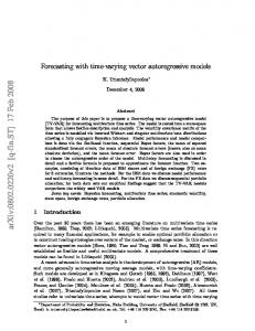
First, in contrast to Table 1, the OLS estimates of the o¤-diagonal coe¢ cients are now severely biased. For example, in Panel B the OLS estimate of 12 is 0.1728 compared to the true value of 0.108. 12 is the coe¢ cient on the lagged dividend-price ratio in the return equation and, hence, measures the degree of stock return predictability by the dividend-price ratio. The large upward bias is due to the large negative correlation between the innovations, which is consistent with e.g. Stambaugh (1999) who studies the e¤ect of small-sample bias on return predictability in a restricted VAR(1) system where 11 = 21 = 0. Based on Kendall’s (1954) bias formula for an AR(1) process, Stambaugh shows that the bias in the OLS estimate of 12 has the opposite sign to the sign of the innovation correlation, which in this case is highly negative. Engsted and Pedersen (2010) show that this conclusion does not hold in general for a multivariate system. Based on a VAR(1) system consisting of the return on a 90-day T-bill, excess returns on stocks and bonds, short nominal yield, log dividend-price ratio, and term spread, they …nd using the analytical bias formula that the bias can in fact have the opposite sign compared to the univariate case. In other words, in the multivariate case the entire correlation structure has an impact on the sign and size of the bias. Regarding the bias in the estimate of 12 , Table 2 also shows that in small samples (Panel B) neither ABF nor BOOT is able to completely eliminate the bias. And this in spite of a relatively low persistence in the dividend-price ratio. Hence, even after correcting for bias there is still a risk of overstating the degree of stock return predictaility by the dividend-price ratio. The second di¤erence in Table 2 compared to Table 1 is that the variances of the bias correction methods are now larger than that of OLS. This prompts the questions: What has caused this relative change in variances, and can the change imply a larger RMSE when correcting for bias than when not? Regarding the …rst question, the relative change in variances is a consequence of the change in (and not u ). In Table 1 both variables in the VAR(1) system are fairly persistent, while in Table 2 this is only the case for the second variable. The relative change in variance is clear from Figure 1, which in the left-hand panel shows the variance of OLS, WLS, and ABF as a function of 11 with the remaining slope coe¢ cients equal to those used in Table 1. The variance is calculated as the average variance across the four slope coe¢ cients based on 10,000 simulations with T = 100. For 11 smaller (larger) than roughly 0:4 the variance of OLS is smaller (larger) than the variance of ABF. Furthermore, the …gure shows that for all values of 11 WLS yields the largest variance. Regarding the second question, the right-hand panel of Figure 1 shows that the RMSE for ABF remains below that of OLS for all values of 11 . Hence, despite a smaller variance for certain values of 11 , the larger bias using OLS results in 12
a higher RMSE than in the case of ABF.5
3.2
Iteration in the analytical bias formula
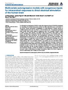
The procedure used to adjust for bias based on the analytical bias formula is very simple and easy to use, since it only requires substituting the biased OLS estimates into bP in (7) to obtain an estimate of the bias which we can then subtract from the OLS estimates. However, since the bias formula holds for the true values of the VAR parameters it is possible that we can obtain estimates with smaller bias if we use a more elaborate iterative scheme in which we repeatedly substitute bias-adjusted estimates into the analytical bias formula. This issue is also relevant when using Chen and Deo’s (2010) weighted least squares estimator. In a simulation study, Chen and Deo use what they call the iterated weighted least squares estimator. They obtain this estimator by …rst using the ordinary least squares estimator in (8), and then by inserting this result back into (8). In this section we compare the simple ’plug-in’approach for the analytical bias formula and the weighted least squares estimator to a more elaborate iterative approach both in terms of bias and variance. The use of an iterative scheme in the analytical bias formula is only relevant if the bias varies as a function of . Figure 2 shows the bias as a function of 22 in a bivariate VAR(1) system with the remaining slope coe¢ cients equal to those used in Table 1. As expected the bias function varies most for small sample sizes, but even for T = 50 the bias function for 11 is relatively ‡at. For 12 and 21 the bias function is relatively steep when the sample size is small and the second variable in the system is fairly persistent. For 22 the bias function is mainly downward sloping. Overall, Figure 2 suggests that the use of an iterative scheme could potentially be useful if the sample size is small, while for larger sample sizes the gain appears to be limited. Of course these plots depend on and the correlation between the innovations. The relatively steep bias functions for 12 and 21 when the sample size is small and the second variable in the system is fairly persistent suggest that if the o¤-diagonal coe¢ cients are of special interest, such as in the case of evaluating return predictability as in Table 2, using an iterative scheme could potentially prove useful. However, the very steep bias function for 12 and 21 is only present when both variables in the system are fairly persistent, and this is not the case in the bivariate system consisting of returns and the dividend-price ratio, since returns 5 We have made similar plots for other sample sizes, but the conclusions remain the same so to conserve space we do not show them here.
13
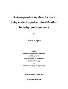
usually have a small autoregressive coe¢ cient. To illustrate the e¤ect of changing and u , Figure 3 shows the bias functions when 11 = 0:1 and the correlation between the innovations is 0:9 but the remaining parameters are identical to those in Figure 2. These parameter choices match fairly well those in Table 2 based on annual log returns and the log dividend-price ratio from S&P data.6 Comparing Figure 3 with Figure 2 it is clear that the bias functions are quite di¤erent. For example, all the bias functions are now very ‡at when the second variable is highly persistent. This means that in terms of evaluating return predictability, iteration is not expected to yield a large gain when correcting for bias. The iterative scheme applied here is basically an extension of the simple ’plug-in’ approach. For the analytical bias formula we, …rst, reestimate the covariance matrix of the innovations, u , after adjusting for bias using the ’plug-in’ approach and then substitute this covariance matrix into the formula together with the bias-adjusted slope coe¢ cients obtained from the ’plug-in’approach. This yields another set of bias-adjusted estimates, which we can then use to reestimate the covariance matrix and the bias. We continue this procedure until the slope coe¢ cient estimates converge. The convergence criteria used here is that the maximum di¤erence across the slope coe¢ cients between two consecutive iterations must be smaller than 10 4 .7 In the ’plug-in’ approach we check if the bias-adjusted estimates are in the stationary region of the parameter space, and if not, we follow Kilian (1998) to ensure that we always get a stationary VAR system. In the iterative scheme we also check for stationarity at each iteration, and if the system contains unit or explosive roots we use Kilian’s procedure and terminate the iterative procedure. Hence, if the VAR system falls into the non-stationary region during the iterative procedure, we will not obtain convergence in the estimates. The iterative approach for the weighted least squares estimator follows the same scheme, with the exception that we do not check for stationarity. An important issue in applying an iterative scheme when using the analytical bias formula is how to treat the covariance matrix of Xt , x . In Section 3.1 we calculated this covariance matrix as vec( x ) = (Ik k ) 1 vec( u ), which implies that we can also reestimate x for each iteration based on the ’new’estimates of and u . Alternatively, 6
We have also made the plots for the VAR(1) models in Table 2 and they are more or less identical to those in Figure 3. Note that only the correlation between the innovations has an impact on the bias, not the variances. 7 Amihud and Hurvich (2004) and Amihud et al. (2009) also use an iterative scheme in their application of the analytical bias formula. However, they use a …xed number of iterations (10) while we iterate until convergence. Convergence is usually obtained within a small number of iterations (4-6), but in a few cases around 20 iterations are needed for the coe¢ cients to converge.
14
we can leave x unchanged throughout the iterative procedure. It is not obvious which strategy yields the best …nite-sample properties and, hence, we examine both approaches in this section. Table 3 shows the results based on 10,000 simulations using the same VAR(1) model as in Table 1. Data are generated as described in Section 3.1. For ease of comparison the table also contains the results based on the simple ’plug-in’approach as reported in Table 1. Regarding WLS, Table 3 shows that iteration reduces the bias but increases the variance. Only for T = 50 is the bias reduction of a su¢ cient magnitude to o¤set the increase in variance implying a decrease in RMSE. For T 100 RMSE increases when iterating on Chen and Deo’s (2010) weighted least squares estimator. For the analytical bias formula with reestimation of x (ABF), iteration yields an improvement over the simple ’plug-in’approach both in terms of bias and variance when T 100. The bias reduction is, however, only present in 11 and 22 (results not shown). In fact, bias in the o¤-diagonal coe¢ cients increase in contrast to what we might expect based on the very steep bias functions in Figure 2. Although the increase is fairly small this illustrates a potential pitfall in iterating on the analytical bias formula in a multivariate setup. For larger sample sizes there is no gain by iterating, which is consistent with the relatively ‡at bias functions displayed in Figure 2. Iterating on the analytical bias formula without reestimating x (ABF ) yields rather di¤erent results. First, using this approach yields a bias function that is not monotonically decreasing in sample size. Note also that for T = 50 the bias is smaller than for both the ’plug-in’procedure and the iterative procedure with reestimation of x , while for T 100 it is larger. Second, the variance is much higher. Combined, these results imply that this procedure yields a higher RMSE than when reestimating x and when using the simple ’plug-in’ approach. Another important di¤erence between the two iterative procedures is that the VAR system much more frequently ends up in the non-stationary region of the parameter space when x is not reestimated.
3.3
Bias-correction in nearly non-stationary models
Although the true VAR system is stationary, we often face the risk of …nding unit or explosive roots when estimating the system based on a …nite sample. In Table 1 for T = 50 we found that in 25 out of 10,000 simulations, OLS yields a non-stationary system. When correcting for bias using either the analytical bias formula or a bootstrap procedure this number increases considerably. However, in these cases we can apply 15
the approach by Kilian (1998) to ensure a stationary system. These results prompt two questions. First, how should we tackle bias-correction if the use of OLS leads to a nonstationary system when we know or suspect (perhaps based on economic theory) that the true VAR system is stationary? Second, how does the use of Kilian’s approach a¤ect the …nite-sample properties of the bias-correction methods? Regarding the …rst question, an alternative to OLS is to use the Yule-Walker (YW) estimator, which is guaranteed to ensure a stationary system. However, YW has a larger bias than OLS and, hence, the …nite-sample properties might be considerably worse. Pope (1990) derives the bias of the YW estimator of the slope coe¢ cient matrix in (2) as bY W BTY W = + O T 3=2 ; (9) T where " # k X 1 2 0 1 0 1 1 bY W = + u (Ik ) + 0 Ik ( 0 ) + (10) i (Ik i ) x : i=1
denotes the i’th eigenvalue of and x is the covariance matrix of Xt . The approach and assumptions are identical to those used by Pope to derive the bias of the OLS estimator.8 Comparing this result to (7) we see that bY W = + bP . In an AR(1) model, yt = + yt 1 + "t , the bias of the YW estimator of can be simpli…ed to (1 + 4 ) =T . Hence, applying YW instead of OLS ensures stationarity but increases the bias. However, since we have an analytical bias formula for the YW estimator we can correct for bias in the same way as we did for OLS. In this section we examine the …nite-sample properties of the YW estimator and compare it to OLS both with and without correction for bias. i
Regarding the question of how the use of Kilian’s approach a¤ect the …nite-sample properties of the bias-correction methods, Kilian’s approach has a practical aim, namely that of ensuring stationary systems. It does not have a theoretical foundation and some deem it to be ad hoc (e.g. Sims and Zha, 1999). The important question from a practical perspective is, however, not whether the approach is theoretically grounded but if we distort the …nite-sample properties by applying it.9 8
Tjøstheim and Paulsen (1983) obtain a similar expression for the bias of the Yule-Walker estimator, but under the assumption of Gaussian innovations. 9 As Kilian (1998) points out, the approach has no e¤ect asymptotically and does not restrict the parameter space of the OLS estimator. However, it will a¤ect the …nite-sample properties and the question is: by how much?
16
Table 4 reports simulation results for the following VAR(1) model " # 0 = ; 0
"
# 0:80 0:10 = ; 0:10 0:94
u
"
# 2 1 = ; 1 2
where the eigenvalues of are 0.748 and 0.992. This VAR(1) model is also used in a simulation study by Amihud et al. (2009). Data are generated as described in Section 3.1. This VAR(1) model is more persistent than the ones used in Tables 1-3, which increases the risk of estimating a non-stationary model using OLS and entering the non-stationary region of the parameter space when correcting for bias. Panel A shows the …nite-sample properties of the OLS, YW, and WLS estimators. Panel B reports the results when using Kilian’s approach to ensure stationarity when correcting for bias using the analytical bias formulas (7) and (10) (both OLS and YW) and bootstrapping (only OLS), while Panel C shows the corresponding results without applying Kilian’s approach. The sample size is 100.10 From Panel A it is clear that YW has a much larger bias than OLS. This is also the case for the variance and, hence, the RMSE for YW is larger than for OLS. However, in contrast to OLS, YW always results in a stationary system, which implies that it is always possible to adjust for bias using the analytical bias formula. In Table 4, OLS yields a non-stationary model in 250 out of 10,000 simulations. The question now is if using the analytical bias formula for YW yields similar …nite-sample properties as in the case of OLS. Panel B (where the procedure by Kilian, 1998, is applied) shows that this is not the case. YW still has a larger bias than OLS and the variance is more that three times as large. Comparing the results for YW with and without bias correction we see that the bias is clearly reduced by applying the analytical bias formula, but the variance also more than doubles. It is also worth to notice that in 7,055 out of 10,000 simulations the system ends up in the non-stationary region when correcting YW for bias compared to only 3,567 for OLS.11 Until now we have used the approach by Kilian (1998) to ensure a stationary VAR system after correcting for bias. Based on the same 10,000 simulations as in Panel B, Panel C shows the …nite-sample properties without applying Kilian’s approach. For OLS 10
We have done the same analysis for other sample sizes and we arrive at the same qualitative conclusions, so to conserve space we do not report them here. 11 Amihud and Hurvich (2004) and Amihud et al. (2009) use the Yule-Walker estimator in a slightly di¤erent way. In their iterative procedure they …rst estimate the model using OLS, and if this yields a non-stationary system, they reestimate the model using Yule-Walker. However, when correcting for bias they still use the analytical bias formula for OLS.
17
(using both the analytical bias formula and a bootstrap procedure) bias decreases and variance increases slightly when we allow the system to be non-stationary. This result is not surprising. The VAR system is highly persistent and very small changes in can result in a non-stationary system, e.g. if 22 is 0.95 instead of 0.94 the system has a unit root. Hence, when applying Kilian’s approach, we often force the estimated coe¢ cients to be smaller than the true values. In contrast, when we allow the system to be non-stationary some of the estimated coe¢ cients will be smaller than the true values and some will be larger and, hence, positive and negative bias will o¤set each other across the 10,000 simulations. Likewise, this will also imply that the variance is larger when we do not apply Kilian’s approach. However, comparing the results for OLS in Panel B and Panel C it is clear that these di¤erences are very small, which implies that Kilian’s approach does not severely distort the …nite-sample properties of the biascorrection methods. And this even though we apply the approach in roughly 4,000 out of 10,000 simulations. In contrast, for YW it turns out to be essential to use Kilian’s approach as seen from Panel C. Note also that allowing the system to be non-stationary (i.e. not applying Kilian’s approach) is not consistent with the fact that the analytical bias formula is derived under the assumption of stationarity.
3.4
Bias-correction when data are skewed and fat-tailed
Until now we have generated data from a multivariate normal distribution. However, in many empirically relevant models the normality assumption often fails. The analytical bias formula is not derived under a normality assumption, but it is unclear how the …nite-sample properties of bias-correction using ABF compare to those of bootstrapping if the data are, for example, very skewed and fat-tailed. Furthermore, in the literature researchers often use a parametric bootstrap based on a normal distribution instead of the usual residual-based bootstrap procedure. The obvious question here is: do we commit errors when using this parametric bootstrap approach when data are very skewed and fat-tailed? In this section, we address these issues. To obtain data that are skewed and has fat tails we estimate a bivariate VAR(1) model containing log returns and log dividend-price ratio on monthly NYSE/AMEX/NASDAQ data from CRSP over the period 1985M1-2008M12. In this period log returns have a skewness of around -1.4 and a kurtosis of approximately 8, while the corresponding numbers for the log dividend-price ratio are 0 and 1.8, respectively. Hence, log returns are far from normally distributed, and given our earlier discussion about return predictability 18
it is relevant to evaluate how the di¤erent bias correction procedures compare in this case. Estimating this bivariate VAR(1) model yields =
"
# 0:0558 ; 0:0418
=
"
# 0:126 0:013 : 0:082 0:989
Table 5 shows simulation results based on these values of and , and where the initial values are drawn from the actual data and the innovations are drawn from the residuals instead of from a normal distribution. The sample size is 100.12 Overall, the results in Table 5 are in line with our previous …ndings, namely that OLS yields highly biased estimates, WLS is able to reduce this bias but at the cost of increased variance, and the bias correction methods provide a large bias reduction compared to both OLS and WLS. Comparing ABF and BOOT, we see that similar to the results in Tables 1, 2, and 4, BOOT yields a slightly smaller bias than ABF, but in contrast the variance is now also lowest for BOOT. The di¤erences are, however, very small. In addition to the residualbased bootstrap approach, Table 5 also shows the results when applying a parametric bootstrap procedure based on an assumption of normally distributed data (PARBOOT). Given that log returns are very skewed and fat-tailed we would expect this approach to have inferior properties compared to both the residual-based bootstrap that directly takes into account the non-normality of the data, and the analytical bias formula that is derived without the assumption of normality. Surprisingly, however, the results in Table 5 show the exact opposite. PARBOOT has both smaller bias and lower variance than BOOT (although the di¤erences are very small). A potential explanation for the very small di¤erence between BOOT and PARBOOT is that the bias is mainly driven by the log dividend-price ratio due to its high persistence, and since this variable is close to being normally distributed the two bootstrap procedures give more or less identical results. In other words, the e¤ects of the non-normal distribution of the less persistent return series have no impact in this context. These results lend some support to the use of a parametric bootstrap procedure when data do not match the assumed distribution, but we refrain from making any general conclusions as it cannot be ruled out that data distributed in a di¤erent way would lead to the opposite result. 12
We have done the same analysis for other sample sizes and we arrive at the same qualitative conclusions, so to conserve space, we do not report them here.
19
4
Concluding remarks
In this paper we have analyzed and compared the …nite-sample properties of various methods for bias-correcting parameter estimates in vector autoregressive models. It is well-known that standard OLS estimates of autoregressive parameters are biased in …nite samples, but in the empirical literature using VAR models this is often ignored. In some cases researchers acknowledge the bias but state that bias-correction is complex in multivariate systems and, hence, they refrain from performing the correction. However, the existing literature provides a simple and easy-to-use analytical bias formula, and in this paper we have shown that the …nite-sample properties of this formula in terms of bias and mean squared error are comparable to those of a more computer-intensive bootstrap procedure. We have also shown that the analytical and bootstrap bias-correction yield a very large reduction in bias compared to both OLS and a recently developed reducedbias estimator by Chen and Deo (2010). In some cases we …nd that the variance of the bias-adjusted estimates is larger than the variance of the OLS estimates, but due to the large reduction in bias the mean squared errors of the bias-adjusted estimates are always smaller than the mean squared errors of the OLS estimates. Hence, through the use of the analytical bias formula correcting for bias in multivariate systems is very simple and without deterioration of …nite-sample properties. We have also analyzed the analytical bias formula in terms of a comparison of a simple one-step ’plug-in’ approach, where the initial least squares estimates are used in place of the true unknown values to obtain the bias-adjusted estimates, and a more elaborate multi-step iterative scheme where we repeatedly substitute bias-adjusted estimates into the bias formulas until convergence. The iterative procedure can potentially yield a smaller bias than the one-step ’plug-in’approach if the bias varies as a function of the slope coe¢ cient matrix. We have shown that the bias functions are highly sensitive to both the slope coe¢ cient matrix and the covariance matrix of the innovations and, hence, it is not clear from the outset how the iterative procedure compares to the ’plug-in’ approach. In a simulation study we have found that iterating on the bias formula results in minor improvements for very small sample sizes while for larger sample sizes there is no gain by iterating. An important issue when correcting for bias is the potential risk of pushing an otherwise stationary model into the non-stationary region of the parameter space, especially if the true system is nearly non-stationary. We have used the approach suggested by Kilian (1998) to account for this, so that we always end up with a model without unit 20
or explosive roots. Although this approach has no e¤ect asymptotically it is unclear how it will a¤ect the …nite-sample properties. In this paper we have shown that the use of Kilian’s approach leads to a very small increase in bias but also a decrease in variance implying a basically una¤ected mean squared error compared to the case where we allow the model to be non-stationary. Hence, it is possible to ensure stationarity through the use of Kilian’s approach without distorting the …nite-sample properties. We have also examined the …nite-sample properties of the Yule-Walker estimator both with and without correcting for bias. In contrast to OLS this estimator is guaranteed to deliver stationary roots but this feature comes at the price of much worse …nite-sample properties both in terms of bias and variance. This is the case both with and without bias-correction. Finally, we have analyzed the …nite-sample properties of the various bias-correction methods in a bivariate VAR system where one of the variables is highly skewed and has fat tails. This data structure does not overturn the overall conclusion of the paper, namely that the analytical and bootstrap bias-correction methods perform equally well and that they have much better …nite-sample properties than both OLS and the reduced-bias estimator by Chen and Deo (2010).
5
Appendix
In this appendix we show that the Yamamoto-Kunitomo formula (4) is identical to Pope’s formula (7). Based on the VAR(1) model Yt = + Yt
1
+ ut ;
t = 1; :::; T
with var (ut ) = u , Yamamoto and Kunitomo (1984) derive the following expression for the asymptotic bias of the OLS estimator of the slope coe¢ cient matrix BTY K =
bY K +O T T
3=2
;
where b
YK
=
u
1 h X
0 i
0 i
( ) + ( ) tr
i+1
i=0
0 2i+1
+( )
"1 i X i=0
21
i
u
0 i
( )
#
1
:
We can rewrite the in…nite sums in the following way 1 X
i
( 0 ) = (Ik
0
1
)
i=0
1 X
0 2i+1
( )
i=0 1 X i
=
0
1 X
2i
( 0) =
0
2
( 0)
Ik
1
i=0
i
u
( 0 ) = E (Yt
)0 = E [Xt Xt 0 ] =
) (Yt
x
i=0
1 X
0 i
( ) tr
i+1
=
i=0
1 X
i
i+1 1
( 0)
+ ::: +
i+1 k
i=0
=
1
1 X
0 i
i 1
( )
+ ::: +
k
i=0
= =
1
j
i
( 0)
i k
i=0
(Ik
k X
1 X
1
(Ik
0
)
1
j
+ ::: + 0
)
1
k
(Ik
0
k
)
1
;
j=1
where Xt = Yt with = (Ik ) 1 and i denotes the i’th eigenvalue of . This implies that bY K = bP and, hence, the bias formulas by Yamamoto and Kunitomo (1984) and Pope (1990) are identical. Consequently, we can also write the bias of OLS estimator of the intercept BT =
b +O T T
3=2
as
;
where b =
u
"
(Ik
0
)
1
+
0
Ik
2
( 0)
1
+
k X i=1
22
i
(Ik
i
0
)
1
#
1 x
(Ik
)
1
:
6
References
Amihud, Y. and Hurvich, C.M. (2004). Predictive regressions: A reduced-bias estimation method. Journal of Financial and Quantitative Analysis 39, 813-841. Amihud, Y., Hurvich, C.M., and Wang, Y. (2009). Multiple-predictor regressions: Hypothesis testing. Review of Financial Studies 22, 413-434. Bao, Y. and Ullah, A. (2007). The second-order bias and mean squared error of estimators in time series models. Journal of Econometrics 140, 650-669. Bauer, M.D., Rudebusch, G.D., and Wu, J. (2011). Unbiased estimation of dynamic term structure models. Working paper, Federal Reserve Bank of San Francisco. Bekaert, G., Hodrick, R.J., and Marshall, D.A. (1997). On biases in tests of the expectations hypothesis of the term structure of interest rates. Journal of Financial Economics 44, 309-348. Chen, W.W. and Deo, R.S. (2010). Weighted least squares approximate restricted likelihood estimation for vector autoregressive processes. Biometrika 97, 231-237. Davison, A.C. and Hinkley, D.V. (1997). Bootstrap Methods and Their Application. Cambridge University Press. Engsted, T. and Pedersen, T.Q. (2010). Return predictability and intertemporal asset allocation: Evidence from a bias-adjusted VAR model. Working paper, Aarhus University. Engsted, T. and Tanggaard, C. (2001). The Danish stock and bond markets: Comovement, return predictability and variance decomposition. Journal of Empirical Finance 8, 243-271. Engsted, T. and Tanggaard, C. (2004). The comovement of US and UK stock markets. European Financial Management 10, 593-607. Engsted, T. and Tanggaard, C. (2007). The comovement of US and German bond markets. International Review of Financial Analysis 16, 172-182. 23
Horowitz, J.L. (2001). The bootstrap in econometrics. In: Heckman, J.J. and Leamer, E.E. (Eds.), Handbook of Econometrics 5, 3159-3228. Kendall, M.G. (1954). Note on the bias in the estimation of autocorrelation. Biometrica 41, 403-404. Kilian, L. (1998). Small-sample con…dence intervals for impulse response functions. Review of Economics and Statistics 80, 218-230. MacKinnon, J.G. and Smith, A.A. (1998). Approximate bias correction in econometrics. Journal of Econometrics 85, 205-230. Marriott, F.H.C. and Pope, J.A. (1954). Bias in the estimation of autocorrelations. Biometrika 41, 390-402. Nicholls, D.F. and Pope, A.L. (1988). Bias in the estimation of multivariate autoregressions. Australian Journal of Statistics 30A, 296-309. Orcutt, G.H. and Winokur, H.S. (1969). First order autoregression: Inference, estimation, and prediction. Econometrica 37, 1-14. Patterson, K.D. (2000). Bias reduction in autoregressive models. Economics Letters 68, 135-141. Pope, A.L. (1990). Biases of estimators in multivariate non-gaussian autoregressions. Journal of Time Series Analysis 11, 249-258. Sawa, T. (1978). The exact moments of the least squares estimator for the autoregressive model. Journal of Econometrics 8, 159-172. Shaman, P. and Stine, R.A. (1988). The bias of autoregressive coe¢ cient estimators. Journal of the American Statistical Association 83, 842-848. Sims, C.A. and Zha, T. (1999). Error bands for impulse responses. Econometrica 67, 1113-1155. 24
Stambaugh, R.F. (1999). Predictive regressions. Journal of Financial Economics 54, 375-421. Tjøstheim, D. and Paulsen, J. (1983). Bias of some commonly-used time series estimates. Biometrika 70, 389-399. White, J.S. (1961). Asymptotic expansions for the mean and variance of the serial correlation coe¢ cient. Biometrika 48, 85-94. Yamamoto, T. and Kunitomo, N. (1984). Asymptotic bias of the least squares estimator for multivariate autoregressive models. Annals of the Institute of Statistical Mathematics 36, 419-430.
25
7
Tables and …gures Table 1. Bias-correction in VAR(1) model, normally distributed innovations. Mean slope coe¢ cients 11
12
21
Bias2
22
Variance RMSE #NS
OLS WLS ABF BOOT
0.7082 0.7441 0.7743 0.7779
0.0906 0.0973 0.0946 0.0963
0.1036 0.1040 0.0995 0.1016
0.7519 0.7927 0.8210 0.8252
0.4538 0.1606 0.0382 0.0281
1.9195 1.9135 1.7520 1.8170
0.1534 0.1438 0.1336 0.1357
25 198 1613 2220
T = 100 OLS WLS ABF BOOT
0.7548 0.7776 0.7931 0.7950
0.0972 0.1019 0.0988 0.1001
0.1035 0.1034 0.1003 0.1015
0.8038 0.8304 0.8433 0.8458
0.1049 0.0225 0.0024 0.0011
0.7324 0.7604 0.6817 0.6965
0.0913 0.0883 0.0826 0.0834
2 18 304 539
T = 200 OLS WLS ABF BOOT
0.7783 0.7924 0.7985 0.7992
0.0995 0.1036 0.1000 0.1005
0.1017 0.1021 0.0999 0.1003
0.8276 0.8449 0.8483 0.8492
0.0245 0.0025 0.0001 0.0000
0.3151 0.3498 0.3013 0.3041
0.0581 0.0592 0.0548 0.0551
0 0 0 2
T = 500 OLS WLS ABF BOOT
0.7917 0.7991 0.8000 0.8002
0.0996 0.1034 0.0998 0.0999
0.1014 0.1025 0.1005 0.1006
0.8407 0.8508 0.8492 0.8494
0.0039 0.0005 0.0000 0.0000
0.1112 0.1316 0.1089 0.1091
0.0339 0.0363 0.0329 0.0330
0 0 0 0
T = 50
The results in this table are based on 10,000 simulations from a VAR(1) model with
=
0 ; 0
=
0:80 0:10 ; 0:10 0:85
u
=
2 1 : 1 2
The eigenvalues are 0.722 and 0.928. For each simulation the initial values are drawn from a multivariate normal distribution with mean (Ik ) 1 and covariance matrix vec( x ) = (Ik k ) 1 vec( u ); and the innovations are drawn from a multivariate normal distribution with mean 0 and covariance matrix u . Bias and variance are multiplied by 100 and together with RMSE they are reported as the average across the four slope coe¢ cients. The …nal column (#NS) gives the number of simulations that result in a VAR(1) system in the non-stationary region. The bootstrap results are based on 1,000 bootstraps. OLS are ordinary least squares estimates; WLS are Chen and Deo (2010) estimates based on equation (8); ABF are bias-adjusted estimates based on the analytical bias formula, equation (7); BOOT are bias-adjusted estimates based on the bootstrap.
26
Table 2. Bias-correction in VAR(1) model for US returns and dividend-price ratio. Mean slope coe¢ cients 11
12
21
22
Bias2
Variance RMSE #NS
Panel A, T = 138 OLS WLS ABF BOOT
0.1057 0.0890 0.0985 0.0981
0.1031 0.0805 0.0820 0.0807
0.1647 0.1946 0.1832 0.1840
0.8607 0.8957 0.8926 0.8948
0.0564 0.0043 0.0005 0.0001
0.5641 0.6621 0.5847 0.5897
0.0760 0.0762 0.0726 0.0729
0 3 12 28
Panel B, T = 63 OLS WLS ABF BOOT
0.1074 0.0782 0.0880 0.0887
0.1728 0.1250 0.1223 0.1178
-0.0599 -0.0262 -0.0354 -0.0360
0.8589 0.9105 0.9128 0.9178
0.2515 0.0184 0.0109 0.0052
1.0567 1.2067 1.1315 1.1351
0.1138 0.1052 0.1038 0.1037
19 169 1090 1532
The results in this table are in Panel A based on 10,000 simulations from a VAR(1) model with
=
0:310 ; 0:346
=
0:098 0:080 ; 0:185 0:896
u
=
0:028837 0:028323
0:028323 ; 0:038776
and a sample size of 138, and in Panel B
=
0:422 ; 0:248
=
0:087 0:108 ; 0:034 0:928
u
=
0:025488 0:023920
0:023920 ; 0:025485
and a sample size of 63. The eigenvalues in Panel A are 0.080 and 0.914, and in Panel B they are 0.091 and 0.924. The VAR(1) models are obtained by estimating a bivariate model containing log returns and log dividend-price ratio on annual S&P data from Robert Shiller’s website. In Panel A the sample period is 1871-2008 and in Panel B it is 1946-2008. For each simulation the initial values are drawn from a multivariate normal distribution with mean (Ik ) 1 and covariance matrix vec( x ) = (Ik k ) 1 vec( u ); and the innovations are drawn from a multivariate normal distribution with mean 0 and covariance matrix u . Bias and variance are multiplied by 100 and together with RMSE they are reported as the average across the four slope coe¢ cients. The …nal column (#NS) gives the number of simulations that result in a VAR(1) system in the non-stationary region. The bootstrap results are based on 1,000 bootstraps. OLS are ordinary least squares estimates; WLS are Chen and Deo (2010) estimates based on equation (8); ABF are bias-adjusted estimates based on the analytical bias formula, equation (7); BOOT are bias-adjusted estimates based on the bootstrap.
27
Table 3. Bias-correction in VAR(1) model, ’plug-in’and iterative scheme. 2
Bias
Plug-in Variance RMSE #NS
2
Bias
Iteration Variance RMSE #NS
WLS ABF ABF
0.1606 0.0382 -
1.9135 1.7520 -
0.1438 0.1336 -
198 1613 -
0.0511 0.0284 0.0224
1.9831 1.7090 2.1451
0.1423 0.1317 0.1470
612 1652 9542
T = 100 WLS ABF ABF
0.0225 0.0024 -
0.7604 0.6817 -
0.0883 0.0826 -
18 304 -
0.0011 0.0016 0.0389
0.8679 0.6745 0.8053
0.0930 0.0821 0.0917
92 304 8331
T = 200 WLS ABF ABF
0.0025 0.0001 -
0.3498 0.3013 -
0.0592 0.0548 -
0 0 -
0.0017 0.0001 0.0096
0.4460 0.3003 0.3452
0.0667 0.0547 0.0595
2 0 4014
T = 500 WLS ABF ABF
0.0005 0.0000 -
0.1316 0.1089 -
0.0363 0.0329 -
0 0 -
0.0030 0.0000 0.0000
0.1932 0.1089 0.1094
0.0441 0.0329 0.0330
0 0 0
T = 50
The results in this table are based on 10,000 simulations from a VAR(1) model with
=
0 ; 0
=
0:80 0:10 ; 0:10 0:85
u
=
2 1 : 1 2
The eigenvalues are 0.722 and 0.928. For each simulation the initial values are drawn from a multivariate normal distribution with mean (Ik ) 1 and covariance matrix vec( x ) = (Ik k ) 1 vec( u ); and the innovations are drawn from a multivariate normal distribution with mean 0 and covariance matrix u . Bias and variance are multiplied by 100 and together with RMSE they are reported as the average across the four slope coe¢ cients. Plug-in gives the results when inserting the biased least squares estimates in the bias formulas and the weighted least squares estimator. Iteration gives the results when recursively using the bias-adjusted estimates in the bias formulas and the weighted least squares estimator. The iterative procedure is terminated when either the slope coe¢ cient matrix is in the non-stationary region or the maximum di¤erence across the slope coe¢ cients between two consecutive iterations is smaller than 10 4 . WLS and ABF (ABF ) are based on equations (8) and (7), respectively. ABF denotes the results when the covariance matrix of Xt is reestimated in each iteration, while ABF leaves it unchanged throughout the iterative procedure. The …nal column for both plug-in and iteration (#NS) gives the number of simulations that result in a VAR(1) system in the non-stationary region.
28
Table 4. Bias-correction in VAR(1) model, nearly non-stationary system. Mean slope coe¢ cients 11
12
21
Bias2
22
Variance RMSE #NS
Panel A OLS YW WLS
0.7508 0.0885 0.1032 0.8890 0.1290 0.6567 -0.0649 0.1542 0.9582 1.2748 0.7720 0.0941 0.0998 0.9140 0.0374
0.6056 0.6578 0.6364
0.0844 0.1284 0.0804
250 0 1236
Panel B (Kilian) ABF (OLS) ABF (YW) BOOT
0.7813 0.0943 0.7829 0.0922 0.7823 0.0951
0.0968 0.9217 0.0182 0.1105 0.9036 0.0448 0.0986 0.9234 0.0153
0.5585 1.7573 0.5709
0.0745 0.1297 0.0750
3567 7055 4266
Panel C ABF (OLS) ABF (YW) BOOT
0.7872 0.0951 0.8778 0.1465 0.7904 0.0962
0.0958 0.9276 0.0089 0.1522 0.9398 0.2734 0.0980 0.9311 0.0047
0.5599 2 102 0.5785
0.0742 1.4960 0.0750
3567 7055 4266
The results in this table are based on 10,000 simulations from a VAR(1) model with
=
0 ; 0
=
0:80 0:10 ; 0:10 0:94
u
=
2 1 : 1 2
The eigenvalues are 0.748 and 0.992. For each simulation the initial values are drawn from a multivariate normal distribution with mean (Ik ) 1 and covariance matrix vec( x ) = (Ik k ) 1 vec( u ); and the innovations are drawn from a multivariate normal distribution with mean 0 and covariance matrix u . The sample size is 100. Panel A shows the results from estimating the VAR(1) model using ordinary least squares (OLS), Yule-Walker (YW), and Chen and Deo’s (2010) weighted least squares estimator (WLS). Panel B and C show the results when adjusting the ordinary least squares estimate for bias using the analytical bias formula (7) (ABF) and bootstrapping (BOOT), and when adjusting the Yule-Walker estimate for bias using the analytical bias formula (10). In Panel B (in contrast to Panel C) the correction by Kilian (1998) to ensure a stationary VAR system is applied. Bias and variance are multiplied by 100 and together with RMSE they are reported as the average across the four slope coe¢ cients. The …nal column (#NS) gives the number of simulations that result in a VAR(1) system in the non-stationary region. The bootstrap results are based on 1,000 bootstraps.
29
Table 5. Bias-correction in VAR(1) model, skewed and fat-tailed innovations. Mean slope coe¢ cients 11
OLS WLS ABF BOOT PARBOOT
12
0.1350 0.1179 0.1236 0.1255 0.1251
0.0551 0.0273 0.0269 0.0253 0.0247
21
22
-0.0919 -0.0732 -0.0787 -0.0807 -0.0803
0.9451 0.9744 0.9746 0.9764 0.9769
Bias2 0.0975 0.0141 0.0106 0.0080 0.0073
Variance RMSE #NS 0.5549 0.6564 0.5593 0.5567 0.5575
0.0784 0.0727 0.0690 0.0685 0.0684
246 1653 3413 3961 4062
The results in this table are based on 10,000 simulations from a VAR(1) model with
=
0:0558 ; 0:0418
=
0:126 0:013 : 0:082 0:989
The eigenvalues are 0.127 and 0.988. The VAR(1) model is obtained by estimating a bivariate model containing log returns and log dividend-price ratio on monthly NYSE/AMEX/NASDAQ data from CRSP over the period 1985M1-2008M12. For each simulation the initial values are drawn from the actual data and the innovations are drawn from the residuals. The sample size is 100. Bias and variance are multiplied by 100 and together with RMSE they are reported as the average across the four slope coe¢ cients. The …nal column (#NS) gives the number of simulations that result in a VAR(1) system in the non-stationary region. The bootstrap results are based on 1,000 bootstraps. OLS are ordinary least squares estimates; WLS are Chen and Deo (2010) estimates based on equation (8); ABF are biasadjusted estimates based on the analytical bias formula, equation (7); BOOT are bias-adjusted estimates based on the bootstrap. PARBOOT are bias-adjusted estimates based on the bootstrap with normally distributed data.
30
Figure 1. Variance and RMSE.
Variance
RMSE 0.095
1
0.09
0.9
0.085 0.8 0.08 0.7
0.075
0.6
0.07
0.065 0.5 0.06 0.4 0.055 0.3
0.2 -1
0.05
-0.8
-0.6
-0.4
-0.2
0
0.2
0.4
0.6
0.8
1
0.045 -1
-0.8
-0.6
-0.4
-0.2
0
0.2
0.4
The …gure shows the variance and RMSE in the VAR(1) slope coe¢ cients as a function of on 10,000 simulations from a VAR(1) model with
=
0 ; 0
=
0:10 11 ; 0:10 0:85
u
=
0.6
11
0.8
based
2 1 ; 1 2
and T = 100, for OLS (solid line), WLS (dotted line), and ABF (dashed line). For each simulation the initial values are drawn from a multivariate normal distribution with mean (Ik ) 1 and covariance matrix vec( x ) = (Ik k ) 1 vec( u ); and the innovations are drawn from a multivariate normal distribution with mean 0 and covariance matrix u . The variance and RMSE are reported as the average across the four slope coe¢ cients. The variance is multiplied with 100.
31
1
Figure 2. Bias function.
Φ 11
Φ 12
0
0.02
-0.02
0.01
-0.04 0 -0.06 -0.01
-0.08
-1
-0.8
-0.6
-0.4
-0.2
0
0.2
0.4
0.6
-0.02 -1
0.8
-0.8
-0.6
-0.4
-0.2
Φ 21 0.04
0.1
0.02
0.05
0
0
-0.02
-0.05
-0.04 -1
-0.8
-0.6
-0.4
-0.2
0
0
0.2
0.4
0.6
0.8
1
0.2
0.4
0.6
0.8
1
Φ 22
0.2
0.4
0.6
0.8
-0.1 -1
1
-0.8
-0.6
-0.4
-0.2
0
The …gure shows the least squares bias in the VAR(1) slope coe¢ cients as a function of true model has an intercept di¤erent from zero and
=
0:80 0:10 ; 0:10 22
u
=
22
when the
2 1 ; 1 2
for T = 50 (solid line), T = 100 (dotted line), and T = 500 (dashed line). The bias function is calculated using the analytical bias formula (7).
32
Figure 3. Bias function.
Φ 11
Φ 12
0.04
0.15
0.02
0.1
0 0.05 -0.02 0
-0.04 -0.06 -1
-0.8
-0.6
-0.4
-0.2
0
0.2
0.4
0.6
0.8
-0.05 -1
1
-0.8
-0.6
-0.4
-0.2
Φ 21
0
0.2
0.4
0.6
0.8
1
0.2
0.4
0.6
0.8
1
Φ 22
0.06
0.1
0.04 0.05 0.02 0
0
-0.02 -0.05 -0.04 -0.06 -1
-0.8
-0.6
-0.4
-0.2
0
0.2
0.4
0.6
0.8
-0.1 -1
1
-0.8
-0.6
-0.4
-0.2
0
The …gure shows the least squares bias in the VAR(1) slope coe¢ cients as a function of true model has an intercept di¤erent from zero and
=
0:10 0:10 ; 0:10 22
u
=
2 1:8
22
when the
1:8 ; 2
for T = 50 (solid line), T = 100 (dotted line), and T = 500 (dashed line). The bias function is calculated using the analytical bias formula (7).
33