Nov 17, 2013 - Vector Autoregression (VAR) is a widely used method for learning ... lem of estimating stable VAR models in a high-dimensional setting, where ...
arXiv:1311.4175v1 [math.ST] 17 Nov 2013
Estimation in High-dimensional Vector Autoregressive Models Sumanta Basu and George Michailidis Department of Statistics, University of Michigan Abstract Vector Autoregression (VAR) is a widely used method for learning complex interrelationship among the components of multiple time series. Over the years it has gained popularity in the fields of control theory, statistics, economics, finance, genetics and neuroscience. We consider the problem of estimating stable VAR models in a high-dimensional setting, where both the number of time series and the VAR order are allowed to grow with sample size. In addition to the “curse of dimensionality” introduced by a quadratically growing dimension of the parameter space, VAR estimation poses considerable challenges due to the temporal and cross-sectional dependence in the data. Under a sparsity assumption on the model transition matrices, we establish estimation and prediction consistency of `1 -penalized least squares and likelihood based methods. Exploiting spectral properties of stationary VAR processes, we develop novel theoretical techniques that provide deeper insight into the effect of dependence on the convergence rates of the estimates. We study the impact of error correlations on the estimation problem and develop fast, parallelizable algorithms for penalized likelihood based VAR estimates.
1
Introduction
Vector Autoregression (VAR) represents a popular class of time series models in applied macroeconomics and finance, widely used for structural analysis and simultaneous forecasting of a number of temporally observed variables. Unlike structural models, VAR provides a broad framework for capturing complex temporal and cross-sectional interrelationship among the time series. In addition to economics, VAR models have been instrumental in linear system identification problems in control theory, while more recently, they have become standard tools in genomics for reconstruction of regulatory networks (Michailidis and d’Alch´e Buc, 2013) and neuroscience for understanding functional connectivity patterns between brain regions. Formally, for a p-dimensional vector-valued stationary time series X t = {X1t , . . . , Xpt }, a VAR model of lag d (VAR(d)) with serially uncorrelated Gaussian errors takes the form i.i.d
X t = A1 X t−1 + . . . + Ad X t−d + �t , �t ∼ N (0, Σ� )
(1.1)
where A1 , . . . , Ad are p × p matrices and �t is a p-dimensional vector of possibly correlated innovation shocks. In the classical setting, estimation of VAR models is undertaken under the assumption P that the process is stable, i.e., det(Ip − dt=1 At z t ) 6= 0 for all z ∈ C, |z| ≤ 1. Note that stability
1
guarantees stationarity. For further discussion on stability we refer the reader to L¨utkepohl (2005). The main objective in VAR models is to estimate the order of the model d and the transition matrices A1 , . . . , Ad . The structure of the transition matrices provide insight into the complex temporal relationships amongst the p time series and lead to efficient forecasting strategies. In many analyses, a second goal is to estimate the error correlations. The matrix Σ� captures the correlation between unknown idiosyncratic errors, which are attributed to additional contemporaneous dependency among the time series. VAR models can also be represented as directed graphs with a partial order (induced by time) among the nodes. Figure 1 depicts a representation of (1.1) with (d + 1)p nodes. The transition matrix of lag j (Aj ) is precisely the adjacency matrix of the bipartite subgraph corresponding to the nodes {X t−j , X t }. If the error process is Gaussian, Σ−1 � corresponds to an undirected graph of additional contemporaneous interaction among the p time series. The directed graphical model
Figure 1: Graphical representation of the VAR model (1.1): directed edges (solid) correspond to the entries of the transition matrices, undirected edges (dashed) correspond to the entries of Σ−1 � induced by the adjacency matrices A1 , . . . , Ad is commonly known as a network of “Grangercausality”. It should be noted that this network, often learned from observational data, merely captures the transition patterns and true causal inference can be drawn only under stringent assumptions. The advent of novel data collection and storage technologies in macroeconomics and finance has enabled researchers to study the relationship amongst a large number of time series. In addition to better forecasting performance, large VAR models also provide better insight into the structure of the economy. For example, Christiano et al. (1999) argues that the increase in price level shortly followed by unexpected monetary tightening, commonly known as “price puzzle”, is an artifact of not including forward looking variables in the model. Also in financial applications, it is often necessary to analyze a large number of time series simultaneously. The problem is that the dimensionality of VAR models grows quadratically with p. For example, estimating a VAR(10) model with p = 10 time series requires estimating dp2 = 1000 parameters. However, it is often very difficult, to obtain a comparable number of stationary observations. Common approaches to deal with this “curse of dimensionality” is to apply shrinkage on the coefficients of the transition matrices or impose some low-dimensional structural assumption on the
2
Xt−2 1
Xt−1 1
●
●
Xt1
α
●
β
− α2
2α
●
X
α ●
●
●
Xt−2 2
Xt−1 2
Xt2
(a) VAR(1) model with p = 2
t−2
●
●
Xt−1
Xt
(b) VAR(2) model with p = 1
β 5
(α, β): {Xt} stable
3 ~ ||A1||
2
α −3
−2
−1
1
2
~ ||A1|| = 1
(α, β): ||A1|| < 1
α
0 −5
−1
0
1
(d) Stability and kA˜1 k < 1
(c) Stability and kA1 k < 1
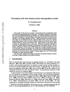
Figure 2: In the left panel, we consider a VAR(1) model with p = 2, X t = A1 X t−1 + �t , where A1 = [α 0; β α]. The unbounded set (dotted) denotes the values of (α, β) for which the process is stable. The bounded region (solid) represents the VAR models that satisfy kA1 k < 1. In the right panel, we consider a VAR(2) model with p = 1, X t = 2αX t−1 − α2 X t−2 + �t . Equivalent formulation of this model as VAR(1) is: Y t = A˜1 Y t−1 + �˜t , where Y t = [X t , X t−1 ]0 , A˜1 = [2α − α2 ; 1 0], and �˜t = [�t , 0]0 . The model is stable whenever |α| < 1 but kA˜1 k is always greater than or equal to 1. VAR model. Bayesian shrinkage is the most popular among such approaches (Ba´nbura et al., 2010)
3
due to its simple implementation and good forecasting performance. In the econometrics literature, a common structural assumption is the presence of few underlying factors, driving economic or market behavior. These assumptions can be incorporated through factor models or principal component analysis. However none of these methods are capable to undertake variable selection. Recent developments in high-dimensional statistics provide a framework to incorporate different lower-dimensional structural assumptions in the model using penalized estimation techniques (e.g., by invoking lasso, group lasso penalties, or low-rank etc.). The simplest of these structures is to assume sparsity on the edge set of the underlying graphical model. This is incorporated in the VAR model by optimizing an `1 -penalization procedure like lasso . Accurate, interpretable, computationally attractive - lasso has received a lot of attention over the past decade in the Statistics community. In a recent work De Mol et al. (2008) have shown that lasso and ridge penalized estimates often provide forecasting accuracy that is comparable to principal component regressions. Studying the theory of VAR estimation in the high-dimensional regime poses considerable challenge due to the dependence between the rows and columns of the design matrix, its crossdependence with the vector of errors and also the dependence among the columns of the error matrix in the multiple regression. Some early attempts to establish consistency of VAR models under high-dimensional scaling include Song and Bickel (2011) and Kock and Callot (2012). Both papers rely on certain regularity assumptions but do not investigate their validity in the context of VAR. Recent works of Negahban and Wainwright (2011) and Loh and Wainwright (2012) provide a more in-depth analysis of the dependence and prove estimation consistency of VAR(1) models under the assumption kA1 k < 1, where k.k denotes the operator norm of a matrix. We show that even this assumption is restrictive and cannot accommodate all stable VAR(1) models. More importantly, as shown in Appendix D, these techniques cannot be directly adapted to VAR(d) model for d > 1, where the dependence structure is more involved. We illustrate this in Figure 2 with two examples. The theoretical properties of the penalized likelihood based estimates have not been addressed before. We provide a unified theory of the least-squares and log-likelihood based VAR estimates which can accommodate any stable VAR(d) model, for any d ≥ 1. This is accomplished by introducing some novel techniques to quantify the unique dependence structure in VAR processes and proving sharp concentration bounds. Our results exploit the spectral properties of stationary VAR processes and provide additional insight into the effect of dependence on the convergence rates of the estimators. Two issues need careful consideration in penalized estimation - (a) choice of loss function (least squares, negative log-likelihood, some other type of divergence etc.), (b) form of penalty (a structural assumption that is relevant to the context of the application and translates to a scalable optimization problem). The second issue, i.e., choice of penalty, is an active area of research in Statistics. Choice of loss function, however, has received less attention in the literature of highdimensional linear regression, primarily because the response is univariate. In VAR settings, one deals with prediction of multiple responses and we show that the choice of loss function can play an important role in the modeling strategy. The standard way to incorporate the sparsity assumption is to penalize the least square objective function (`1 -LS). This estimate does not account for the contemporaneous correlation (Σ� ) among the errors (see Figure 1). In a recent paper Davis et al. (2012) showed that a penalized log-likelihood based approach (`1 -LL), which takes into account the structure of Σ� , sometimes performs better than `1 -LS. The proposed estimator is a maximum likelihood estimate of Ah , assuming Σ� is known. Maximizing the complete likelihood (`1 -ML) with respect to Ah , Σ� poses additional challenge as it involves estimating both the transition matrices Ah and a high-dimensional inverse covariance matrix Σ−1 � . In this work we provide theoretical results for the first two estimates and compare their
4
performances numerically. Computation of the penalized least-square estimates (`1 -LS) of large VAR is straightforward since the estimation problem can be decomposed into p separate LASSO programs and computation can be carried out in parallel. Computing the likelihood based estimators `1 -LL and `1 -ML, however, needs more work since the regressions are not separable. For example, the algorithm presented in Davis et al. (2012) does not take advantage of parallel computing when p is large. To this end, we propose a blockwise coordinate descent algorithm that is parallelizable and is of the same order of complexity as `1 -LS. In summary, the main contributions of this work are: (a) develop novel theoretical techniques to analyze penalized estimators for high-dimensional stable, Gaussian VAR model of any order d, (b) investigate analytically the properties of least square and likelihood based methods in the highdimensional regime, and (c) develop parallellizable algorithm for likelihood based VAR estimates.
2
Modeling Framework
Consider a single realization of {X 0 , X 1 , . . . , X T } generated according to a p-dimensional vector autoregressive model of order d with serially uncorrelated Gaussian errors X t = A1 X t−1 + . . . + Ad X t−d + �t , �t ∼N (0, Σ� ), Cov(�t , �s ) = 0p×p if t 6= s
(2.1)
Throughout the paper we will assume that the error covariance matrix Σ� is positive definite so that Λmin (Σ� ) > 0 and Λmax (Σ� ) < ∞. Here Λmin and Λmax denote the minimum and maximum eigenvalues of a symmetric or hermitian matrix, respectively. We will also assume that the VAR P process is stable, i.e., all the eigenvalues of the reverse characteristic polynomial A(z) = Ip − dt=1 At z t lie outside the unit circle {z ∈ C : |z| = 1}. Formally, d X det(A(z)) = det(Ip − At z t ) 6= 0, for all |z| ≤ 1 (2.2) t=1
The stability of the process guarantees that all the eigenvalues of the Hermitian matrix A∗ (z)A(z) are positive, whenever |z| = 1. We take the following quantity as a measure of stability of the VAR(d) process: µmin (A) = min Λmin (A∗ (z)A(z)) |z|=1
We also define a second, related quantity that will be useful in our theoretical analyses: µmax (A) = max Λmax (A∗ (z)A(z)) |z|=1
Note that µmin (A) and µmax (A) are well-defined because of the continuity of eigenvalues and compactness of the unit circle {z ∈ C : |z| = 1}. Further, stability of the process guarantees that these are positive. We will often use an equivalent representation of a VAR(d) model. This states that a p-dimensional ˜ t = A˜1 X ˜ t−1 + �˜t VAR(d) process (2.1) can be represented as a dp-dimensional VAR(1) process X
5
with ˜t = X
Xt X t−1 .. .
X t−d+1
A˜1 =
dp×1
··· ··· ··· .. .
A1 A2 Ip 0 0 Ip .. .. . . 0 0
···
t Ad−1 Ad � 0 0 0 0 0 �˜t = . .. .. .. . . 0 Ip 0 dp×dp
(2.3)
dp×1
˜ t with reverse characteristic polynomial A(z) ˜ In view of (2.2), the process X := Idp − A˜1 z is stable t if and only if the process X is stable. However, the stability measures µmin (A), µmax (A) are not ˜ µmax (A). ˜ necessarily the same as µmin (A), A key ingredient of our frequency domain analysis is the spectral density matrix of the VAR process (2.1), defined as f (θ) =
∞ 1 X Γ(l)e−ilθ , 2π
θ ∈ [−π, π]
(2.4)
l=−∞
� � where Γ(l) = E X t (X t+l )0 denotes the autocovariance matrix of order l. If the process is stable, the spectral density matrix has the following closed form expression (cf. equation (9.4.23), Priestley (1981)) �−1 � �−1 1 � A(e−iθ ) f (θ) = Σ� A∗ (e−iθ ) (2.5) 2π The quantities µmin (A), µmax (A), Λmin (Σ� ) and Λmax (Σ� ) play important roles in our theoretical analysis. Essentially, these quantities determine some upper and lower bounds on the extreme eigenvalues of the spectral density matrix and help capture the effect of temporal and cross-sectional dependence on the VAR estimates. As seen in Figure 1, dependence in a VAR process comes from two distinct sources: (a) the transition matrices A1 , . . . , Ad and (b) the error covariance Σ� . In time domain analysis it is difficult to separate the two sources. In frequency domain analysis, however, this is accomplished very easily, as seen in (2.5). This leads to tighter control of the dependence and sharper concentration bounds. In Appendix D we provide some useful bounds on the stability measures and discuss their connection with the assumption kAk < 1.
2.1
Notation.
Based on the data {X 0 , . . . , X T }, we construct autoregression (X T )0 (X T −1 )0 · · · (X T −d )0 .. .. .. .. = . . . . d 0 d−1 0 0 0 (X ) (X ) ··· (X ) | {z } {z }| | Y
X
T 0 (� ) A01 .. + .. . . A0d (�d )0 {z } | {z B∗
E
}
vec(Y) = vec(X B) + vec(E) = (I ⊗ X ) vec(B ∗ ) + vec(E) Y |{z}
N p×1
=
Z β ∗ + vec(E) |{z} |{z} | {z }
N p×q q×1
N p×1
6
N = (T − d + 1), q = dp2
(2.6)
P We will assume that β ∗ is a k-sparse vector, i.e., dt=1 kAt k0 = k. We denote the (i, j)th entry of Σ and Σ−1 by σ�,ij and σ�ij , respectively. For any matrix M , we use Mj to denote its j th column. We use kAk to denote the `2 -norm when A is a vector and the operator norm when A is a matrix. Any other choice of norm is mentioned explicitly. We use ei to denote the ith unit vector in RN .
2.2
Estimates.
We consider two different estimates for the transition matrices A1 , . . . , Ad , or equivalently, for β ∗ . The first one is an `1 -penalized least squares estimate of VAR coefficients (`1 -LS). It is defined as argmin β∈Rq
1 kY − Zβk2 + λN kβk1 N
(2.7)
This estimate does not exploit the error covariance structure Σ� . The second one uses an `1 -penalized log-likelihood estimation (`1 -LL). This is defined as argmin β∈Rq
� 1 (Y − Zβ)0 Σ−1 � ⊗ I (Y − Zβ) + λN kβk1 N
(2.8)
This is a maximum likelihood estimate of β, assuming the error covariance Σ� is known. Although it is not directly applicable in practice, we study the properties of this estimate to demonstrate some important aspects related to the choice of loss function. In section 3, we implement this method with a plug-in estimate of Σ� , obtained using the residuals from an ordinary least squares or `1 -LS fit. A third estimate, `1 -penalized maximum-likelihood estimate of VAR coefficients (`1 -ML), can be formulated as argmin p×p β∈Rq ,Σ−1 � ∈R
� 1 −1 −1 (Y − Zβ)0 Σ−1 � ⊗ I (Y − Zβ) − log det(Σ� ) + λN kβk1 + Pγ (Σ� ) (2.9) N
It maximizes the full likelihood with respect to (β, Σ−1 � ) under an `1 -regularization on β and some . The second penalty can be chosen appropriately to incorporate some convex penalty Pγ on Σ−1 � relevant structural assumption (sparsity, block structure etc.) on Σ−1 � . Theoretical analysis of this estimate is more involved than the previous ones as it involves estimating an undirected graph from dependent samples of residuals. In this paper we do not study this estimate theoretically. In section 3 we show that a simple variant of our algorithm for `1 -LL can be used to implement this.
3
Implementation.
The optimization problem `1 -LS in (2.7) can be expressed as p separate penalized regression problems: argmin β∈Rq
1 kY − Zβk2 + λN kβk1 N
p p X 1 X 2 ≡ argmin kYi − X Bi k + λN kBi k1 B1 ,...,Bp N i=1
i=1
7
This amounts to running p separate lasso programs, each with dp predictors: Yi ∼ X , i = 1, . . . , p. For large d and p, the p programs can be solved in parallel. In the optimization problem `1 -LL, the above regressions are coupled through Σ−1 � . One way to solve the problem, as mentioned in Davis et al. (2012), is to reformulate it into a single penalized regression problem: � 1 (Y − Zβ)0 Σ−1 � ⊗ I (Y − Zβ) + λN kβk1 β∈R N � � � � 2 1
−1/2
≡ arg minq ⊗ I Y − Σ−1/2 ⊗ X β + λN kβk1
Σ� � β∈R N � � −1/2 −1/2 This amounts to running a single lasso program with dp2 predictors: Σ� ⊗ I Y ∼ Σ� ⊗X . This is computationally expensive for large d and p. Unlike `1 -LL, this algorithm is not parallelizable. We propose an alternative algorithm based on blockwise coordinate descent to estimate the `1 LL coefficients. To this end, we first observe that the objective function in (2.8) can be simplified to arg
minq
p p p X 1 X X ij 0 σ� (Yi − X Bi ) (Yj − X Bj ) + λN kBk k1 N i=1 j=1
k=1
Minimizing the above objective function cyclically with respect to each Bi leads to the following algorithm for `1 -LL and `1 -ML (the last step is used only for `1 -ML): ˆ Σ ˆ −1 1. pre-select d. Run `1 -LS to get B, � . 2. iterate till convergence: (a) For i = 1, . . . , p, • set ri := (1/2 σ ˆ�ii )
X
� � ˆj σ ˆ�ij Yj − X B
j6=i
ˆ�ii ˆi = argmin σ k(Yi + ri ) − X Bi k2 + λN kBi k1 • update B N Bi ˆ −1 (b) [only for `1 -ML]: update Σ � as argmin p×p Σ−1 � ∈R
p p �0 � � 1 X X ij � −1 ˆi ˆj − log det(Σ−1 σ� Yi − X B Yj − X B � ) + Pγ (Σ� ) (3.1) N i=1 j=1
In this algorithm, a single iteration amounts to running p separate lasso programs, each with dp predictors: Yi + ri ∼ X , i = 1, . . . , p. As in `1 -LS, these p programs can be solved in parallel. Further, for solving `1 -ML, one can incorporate structural information about Σ−1 � (sparsity, block structure, bandedness etc.) using the penalty Pγ (.).
4
Theoretical Properties
In this section we analyze the theoretical properties of the two penalized estimators `1 -LS and `1 -LL, proposed in Section 2. We provide non-asymptotic upper bounds on their estimation and in-sample prediction errors under different choices of norms. First, for a given realization of
8
{X 0 , . . . , X T }, we derive a deterministic upper bound on the errors under standard restricted eigenvalue and deviation conditions. We then show that for a random realization of {X 0 , . . . , X T } generated according to a stable VAR(d) process, these conditions hold with high probability. The first result is known from the literature of high-dimensional linear regressions. The other results, viz., verifying the two regularity conditions for general VAR(d) models, have not been studied before. We analyze the two problems (2.7) and (2.8) under a general penalized M-estimation framework proposed in Loh and Wainwright (2012). To motivate this general framework, note that the VAR estimation problem with ordinary least squares is equivalent to the following optimization 0 0 ˆ argmin −2β γˆ + β Γβ,
(4.1)
β∈Rq
� � � � ˆ = I ⊗ X 0 X /N , γˆ = I ⊗ X 0 Y /N are unbiased estimates for their population where Γ analogues. ˆ in the penalized version of the objective function leads to the A more general choice of (ˆ γ , Γ) following optimization problem 0 0 ˆ + λN kβk , argmin −2β γˆ + β Γβ 1
(4.2)
β∈Rq
� � � � ˆ = W ⊗ X 0 X /N , γˆ = W ⊗ X 0 Y /N Γ where W is a symmetric, positive definite matrix of weights. The optimization problems (2.7) and (2.8) are special cases of (4.2) with W = I and W = Σ−1 � , respectively. Consistent estimation of VAR models in the low-dimensional regime (p, d finite, T → ∞) relies on two assumptions (cf. Section 3.2.2, L¨utkepohl (2005)): (a) X 0 X /N converges in probability to a non-singular matrix C (i.e., Λmin (C) > 0) and (b) vec(X 0 E)/N converges to zero in probability. In the high-dimensional regime (N � q) the first assumption is never true since the design matrix is rank-deficient (more variables than observations). The second assumption is also very stringent since the dimensions of X 0 E grows with N . Interestingly, consistent estimation in the high-dimensional regime can be guaranteed under two analogous sufficient conditions. The first one comes from a class of conditions commonly referred to as Restricted Eigenvalue (RE) conditions. Different variants of the RE condition have been proposed in the literature (Bickel et al., 2009; van de Geer and B¨uhlmann, 2009). Roughly speaking, in the regression framework of (2.6), these assumptions require that kZ(βˆ − β ∗ )k is small ˆ β ∗ are any arbitrary vectors in Rq , this assumption is never true only when kβˆ − β ∗ k is small. If β, since the columns of Z are correlated. However, if β ∗ is sparse and λN is appropriately chosen, it is now well-understood that the vectors βˆ − β ∗ only vary on a low-dimensional subset of the high-dimensional space Rq , with high probability. This indicates that the RE condition may not be very stringent after all, even though the columns of Z are correlated. Although, verifying that the assumption is indeed satisfied with high probability, is often far from trivial. We work with the RE condition proposed in Loh and Wainwright (2012). This is a slightly stronger version of the original RE assumption proposed in (Bickel et al., 2009), as discussed in Raskutti et al. (2010). ˆ satisfies (A1) Lower-Restricted Eigenvalue Assumption (Loh and Wainwright, 2012): Γ restricted eigenvalue condition with curvature α > 0 and tolerance τ (N, q) > 0 if ˆ ≥ α kθk2 − τ (N, q) kθk2 , ∀ θ ∈ Rq θ0 Γθ 1
9
(4.3)
ˆ are well-behaved in the sense that they concentrate The second condition ensures that γˆ and Γ ˆ ∗ have the same expectation, this assumption nicely around their population means. As γˆ and Γβ requires an upper bound on their difference. Note that in the low-dimensional context of (4.1), ˆ ∗ is precisely vec(X 0 E)/N . γˆ − Γβ (A2) Deviation Condition: There exists a deterministic function Q (β ∗ , Σ� ) such that r
log q
∗ ∗ ˆ (4.4)
γˆ − Γβ ≤ Q (β , Σ� ) N ∞ The following proposition establishes non-asymptotic upper bounds on the estimation and prediction errors when the above conditions are satisfied. Proposition 4.1 (Estimation and prediction error). Consider the penalized M-estimation problem ˆ (4.2) with W = I or W = Σ−1 � . Suppose Γ satisfies lower RE condition (4.3) with kτ p(N, q) ≤ ∗ ˆ α/32 and (Γ, γˆ ) satisfies the deviation bound (4.4). Then, for any λN ≥ 4Q(β , Σ� ) log q/N , any solution βˆ of (4.2) satisfies kβˆ − β ∗ k1 ≤ 64 k λN /α √ kβˆ − β ∗ k ≤ 16 k λN /α
(4.5)
(4.6) ∗ 0ˆ ˆ ∗ 2 ˆ (β − β ) Γ(β − β ) ≤ 128 k λN /α (4.7) P Remarks. kβˆ − β ∗ k is precisely dt=1 kAˆt − At kF , the `2 -error in estimating the transition ∗ 0ˆ ˆ ∗ ) is a measure of in-sample prediction error under ` -norm, ˆ matrices. For 2 PT`1 -LS,P(dβ − βˆ ) Γ(β − β t−h ∗ 0ˆ ˆ ∗ ˆ defined as t=d k h=1 (Ah − Ah )X k2 /N . For `√ 1 -LL, (β − β ) Γ(β − β ) takes the form Pd PT t−h k2 /N , where kvk := ˆ v 0 Σ−1 v. This can be viewed as a measure Σ h=1 (Ah − Ah )X t=d k Σ� of in-sample prediction error under a Mahalanobis type distance on Rp induced by Σ� . The convergence rates are governed by two sets of parameters: (i) dimensionality parameters - dimension of the process (p), order of the process (d), number of edges in the network (k) and sample size (N = T-d+1); (ii) intrinsic parameters - restricted eigenvalue(or curvature) (α), tolerance (τ (N, q)) and the deviation bound Q(β ∗ , Σ� ). The squared `2 -errors of estimation and prediction scale with the dimensionality parameters as k(2 log p + log d)/N , same as the rates obtained when the observations are independent (Bickel et al., 2009). The temporal and cross-sectional dependence affect the rates only through the intrinsic parameters. Typically, the rates are better when α is large and Q(β ∗ , Σ� ), τ (N, q) are small. In propositions 4.2 and 4.3 we investigate in detail how these quantities are related to the dependence structure of the process. Although the above proposition is derived under the assumption that d is the true order of the VAR process, the results hold if d is an upper bound on the true order. This follows from the ¯ for any d¯ > d, with transition matrices fact that a VAR(d) model can also be viewed as VAR(d), A1 , . . . , Ad , 0p×p , . . . , 0p×p . Proposition 4.1 is deterministic, i.e., it assumes a fixed realization of {X 0 , . . . , X T }. To show that these error bounds hold with high probability, one needs to verify that the assumptions (A1-2) are satisfied with high probability when {X 0 , . . . , X T } is a random realization from the VAR(d) process. This is accomplished in the next two propositions. Verifying RE assumption. The problem of verifying RE-type assumptions for correlated design matrices has been studied by several authors (Raskutti et al., 2010; Rudelson and Zhou, 2013). These results require independence among the rows of the design matrix and are not directly applicable for VAR models. Verifying RE-type assumptions on a general design matrix where both the rows and columns are dependent is indeed a daunting task. To the best of our knowledge, the
10
closest results are due to Negahban and Wainwright (2011) and Loh and Wainwright (2012). However, their results crucially depend on the assumption kAk < 1 and cannot be extended beyond a subclass of stable VAR(1) models (Figure 2 and Lemma D.2). We have dealt with this challenge by quantifying the uniqe dependence structure in VAR processes through its spectral representation. The results rely on a key technical lemma B.1. Conducting part of our analysis in the frequency domain, we were able to prove sharper concentration bounds that helped verify RE for any stable VAR(d) model, for d ≥ 1. The techniques are fairly general and can be adapted for a broader class of stationary processes and different penalties other than lasso. ˆ Consider a random realization {X 0 , . . . , X T } generated Proposition 4.2 (Verifying RE for Γ). according to a stable VAR(d) process (2.1). Then there exist universal positive constants ci such that for all N % max{1, ω −2 }k log(dp), with probability at least 1 − c1 exp(−c2 N min{ω 2 , 1}), the matrix ˆ = Ip ⊗ (X 0 X /N ) ∼ RE(α, τ ), Γ where ω=
Λmin (Σ� )/Λmax (Σ� ) Λmin (Σ� ) Λmin (Σ� ) log(dp) , α= , τ (N, q) = c3 max{ω −2 , 1} . ˜ 2µ (A) µ (A) N µmax (A)/µmin (A) max max
Further, if Σ−1 ¯�i := σ�ii − � satisfies σ as above, the matrix
ij j6=i σ�
P
> 0, for i = 1, . . . , p, then, with the same probability
� � � −1 0 i i ˆ Γ = Σ� ⊗ X X /N ∼ RE α min σ ¯� , τ (N, q) max σ ¯� i
i
This proposition provides insight into the effect of temporal and cross-sectional dependence on the convergence rates obtained in Proposition 4.1. As mentioned earlier, the convergence rates are faster for larger α and smaller τ . From the expressions of ω, α and τ , it is clear that the VAR estimates have lower error bounds when Λmax (Σ� ), µmax (A) are smaller and Λmin (Σ� ), µmin (A) are larger. We defer the proof to Appendix B. Verifying Deviation Condition. The problem of verifying the deviation condition poses some unique challenges that are specific to VAR models. In the literature of high-dimensional linear regression with random design, one typically assumes that the errors are independent of the design matrix. This does not hold for VAR models since X t is always correlated with �t−1 . In the classical, fixed p analysis of VAR, this is resolved by invoking martingale central limit theorem on the coordinates of X 0 E. In the non-asymptotic, high-dimensional framework, a natural alternative is to come up with sharp martingale concentration inequalities. The standard martingale inequalities involve some measure ofPpredictable quadratic variation (Bercu and Touati, 2008), which, in our T −1 context, corresponds to t=d−1 (Xjt )2 . To establish a meaningful deviation bound, one needs to derive a second concentration bound for this term and somehow combine the two. Although viable, this approach often leads to poor and cumbersome deviation bounds. Interestingly, we found that taking advantage of the spectral representation of VAR helps establish useful concentration bounds required to verify the deviation condition (A2). The main idea is to express the errors in terms of the design matrix and take advantage of the spectral representation of the autocovariance function. The proof relies crucially on a key technical lemma C.1. To the best of our knowledge, this is a novel technique to establish deviation inequalities for high-dimensional autoregressive processes.
11
Proposition 4.3 (Deviation Bound). For any q ≥ 2, A > 0, N % log q, with probability at least 1 − 12q −A , we have r
ˆ ∗ ≤ Q(β ∗ , Σ� ) log q ,
γˆ − Γβ N ∞ where, for `1 -LS, � � p Λmax (Σ� ) Λmax (Σ� )µmax (A) Q(β , Σ� ) = (18 + 6 2(A + 1)) Λmax (Σ� ) + + µmin (A) µmin (A) ∗
and for `1 -LL, ∗
p Q(β , Σ� ) = (18 + 6 2(A + 1))
�
1 Λmax (Σ� ) Λmax (Σ� )µmax (A) + + Λmin (Σ� ) µmin (A) Λmin (Σ� )µmin (A)
�
As before, this proposition shows that the VAR estimates have lower error bounds when Λmax (Σ� ), µmax (A) are smaller and Λmin (Σ� ), µmin (A) are larger.
5
Numerical Experiments
We evaluate the performances of `1 -LS and `1 -LL on simulated data and compare with the performances of ordinary least squares (OLS) and Ridge estimates. Implementing `1 -LL requires an estimate of Σ� in the first step. For this, use the residuals from `1 -LS to construct a plug-in estimate Σˆ� . To evaluate the effect of error correlation on the transition matrix estimates more precisely, we also implement an oracle version, `1 -LL-O, which uses the true Σ� in the estimation. Next, we describe the simulation settings, choice of performance metrics and discuss the results. We design two sets of numerical experiments - (a) SMALL VAR (p = 10, d = 1, T = 30, 50) and (b) MEDIUM VAR (p = 30, d = 1, T = 80, 120, 160). In each setting, we generate an adjacency matrix A1 with 5 ∼ 10% non-zero edges selected at random and rescale to ensure that the process is stable with SN R = 2. We generate three different error processes with covariance matrix Σ� from one of the following families: 1. Block-I: Σ� = ((σ�,ij ))1≤i,j≤p with σ�,ii = 1, σ�,ij = ρ if 1 ≤ i 6= j ≤ p/2, 0 otherwise; 2. Block-II: Σ� = ((σ�,ij ))1≤i,j≤p with σ�,ii = 1, σ�,ij = ρ if 1 ≤ i 6= j ≤ p/2 or p/2 < i 6= j ≤ p, 0 otherwise; 3. Toeplitz: Σ� = ((σ�,ij ))1≤i,j≤p with σ�,ij = ρ|i−j| . We let ρ vary in {0.5, 0.7, 0.9}. Larger values of ρ indicate that the error processes are more strongly correlated. Figure 3 illustrates the structure of a random transition matrix used in our simulation and the three different types of error covariance structure. We compare the different methods for VAR estimation (OLS, `1 -LS, `1 -LL, `1 -LL-O, Ridge) based on the following performance metrics: 1. Model Selection: Area under receiving operator characteristic curve (AUROC) ˆ − BkF /kBkF 2. Estimation error: Relative estimation accuracy measured by kB We report the results for small VAR with T = 30 and medium VAR with T = 120 (averaged over 50 replicates) in Tables 1 and 2. The results in the other settings are qualitatively similar,
12
(a) A1
(b) Σ� : Block-I
(c) Σ� : Block-II
(d) Σ� : Toeplitz
Figure 3: Adjacency matrix A1 and error covariance matrix Σ� of different types used in the simulation studies Table 1: VAR(1) model with p = 10
AUROC
Estimation Error
p = 10 T = 30 `1 -LS `1 -LL `1 -LL-O OLS `1 -LS `1 -LL `1 -LL-O ridge
ρ = 0.5 0.77 0.77 0.8 1.24 0.68 0.66 0.61 0.72
BLOCK-I ρ = 0.7 0.74 0.75 0.79 1.39 0.72 0.66 0.62 0.74
ρ = 0.9 0.7 0.73 0.76 1.77 0.76 0.66 0.62 0.75
ρ = 0.5 0.79 0.79 0.82 1.29 0.64 0.57 0.53 0.7
BLOCK-II ρ = 0.7 ρ = 0.9 0.76 0.74 0.77 0.77 0.8 0.81 1.63 2.36 0.67 0.7 0.59 0.53 0.54 0.47 0.71 0.72
ρ = 0.5 0.82 0.81 0.85 1.32 0.63 0.59 0.53 0.7
Toeplitz ρ = 0.7 0.79 0.8 0.84 1.56 0.66 0.56 0.51 0.71
ρ = 0.9 0.77 0.81 0.84 2.58 0.69 0.49 0.42 0.72
although the overall accuracy changes with the sample size. We find that the regularized VAR estimates outperform ordinary least squares uniformly in all the cases. In terms of model selection, the `1 -penalized estimates perform fairly well, as reflected in their AUROC. Ordinary least squares and ridge regression do not perform any model selection. Further, for all three choices of error covariance, the two variants of `1 -LL outperform `1 -LS. The difference in their performances is more prominent for larger values of ρ. Among the three covariance structures, the difference between least squares and log-likelihood based methods is more prominent in Block-II and Toeplitz family since the error processes are more strongly correlated. Finally, in all the cases, the accuracy of `1 -LL is somewhere in between `1 -LS and `1 -LL-O, which suggests that a more accurate estimation of Σ� might improve the model selection performance of regularized VAR estimates. In terms of `2 -error of estimation, the conclusions are broadly the same. The effect of overfitting is reflected in the performance of ordinary least squares. In many settings, the estimation error of ordinary least squares is even twice as large as the signal strength. The performance of ordinary least squares deteriorates when the error processes are more strongly correlated (see, for example, ρ = 0.9 for block-II). Ridge regression performs better than ordinary least squares as it applies shrinkage on the coefficients. However the `1 -penalized estimates show higher accuracy than Ridge in almost all the cases. This is somewhat expected as the data were simulated from a sparse model with strong signals, whereas Ridge regression tend to favor a non-sparse model with many small coefficients.
13
Table 2: VAR(1) model with p = 30
AUROC
Estimation Error
A
p = 30 T = 120 `1 -LS `1 -LL `1 -LL-O OLS `1 -LS `1 -LL `1 -LL-O Ridge
ρ = 0.5 0.89 0.89 0.92 1.73 0.72 0.71 0.66 0.81
BLOCK-I ρ = 0.7 0.85 0.87 0.9 2 0.76 0.71 0.66 0.83
ρ = 0.9 0.77 0.82 0.84 2.93 0.85 0.72 0.68 0.85
ρ = 0.5 0.87 0.9 0.93 1.95 0.74 0.68 0.64 0.82
BLOCK-II ρ = 0.7 ρ = 0.9 0.81 0.69 0.89 0.88 0.92 0.9 2.53 4.28 0.82 0.93 0.68 0.65 0.63 0.59 0.85 0.88
ρ = 0.5 0.91 0.91 0.94 1.82 0.69 0.67 0.63 0.81
Toeplitz ρ = 0.7 0.87 0.91 0.93 2.28 0.73 0.63 0.59 0.82
ρ = 0.9 0.76 0.89 0.92 3.88 0.86 0.6 0.54 0.86
Results of Consistency
Proof of Proposition 4.1. Since βˆ is a minimizer of (4.2), for all β ∈ Rq we have ˆ 1 ≤ −2β 0 γˆ + β 0 Γβ ˆ βˆ + λN kβk ˆ + λN kβk1 −2βˆ0 γˆ + βˆ0 Γ For β = β ∗ , the above inequality reduces to ˆ v ≤ 2ˆ ˆ ∗ ) + λN {kβ ∗ k1 − kβ ∗ + vˆk1 } vˆ0 Γˆ v 0 (ˆ γ − Γβ
(A.1)
where vˆ = βˆ − β ∗ . p The first term on the right hand side of (A.1) can be upper bounded by 2kˆ v k1 Q(β ∗ , Σ� ) log q/N . The second term, by triangle inequality, is at most λN {kˆ vS k1 − kˆ vS c k1 }, where S denotes the support of β ∗ . Together with the choice of λN , this leads to the following inequality λN {kˆ vS k1 + kˆ vS c k1 } + λN {kˆ vS k1 − kˆ vS c k1 } 2 λN 3λN kˆ vS k1 − kˆ vS c k1 ≤ 2λN kˆ v k1 (A.2) ≤ 2 2 √ In particular, this implies kˆ vS c k1 ≤ 3kˆ vS k1 so that kˆ v k1 ≤ 4kˆ vS k1 ≤ 4 kkˆ v k. This, together with the restricted eigenvalue and the upper bound on kτ (N, q) implies ˆv ≤ 0 ≤ vˆ0 Γˆ
ˆ v ≥ α kˆ vˆ0 Γˆ v k2 − τ (N, q)kˆ v k21 ≥ (α − 16kτ (N, q))kˆ v k2 ≥ ˆ v guarantee that Together, the upper and lower bounds on vˆ0 Γˆ √ α kˆ v k2 ≤ λN kˆ v k1 ≤ 4 kλN kˆ vk 4 This implies √ kˆ v k ≤ 16 kλN /α
√ v k ≤ 64kλN /α kˆ v k1 ≤ 4 kλN kˆ 0ˆ vˆ Γˆ v ≤ 2λN kˆ v k1 ≤ 128kλ2N /α
14
α kˆ v k2 2
B
Results for Restricted Eigenvalue
ˆ = W ⊗ (X 0 X /N ) where W = I for `1 -LS and W = Σ−1 Recall that Γ � for `1 -LL. Since W is deterministic, we first verify RE assumption on the random matrix X 0 X /N and then investigate the ˆ assumptions on W under which the same holds for Γ. 0 ˜ ˜ t ), constructed using N dependent Note that S = X X /N is an estimate for Γ(0) = Var(X d−1 T −1 ˜ ˜ ˜ samples {X ,...,X }. To establish RE on S, one needs to first ensure that Λmin (Γ(0)) > 0. This is accomplished in Lemma B.1. The next step is to ensure that S concentrates nicely around ˜ Γ(0) in an appropriate sense. This task is accomplished in Lemma B.3. In particular, we show ˜ that for any v = βˆ − β ∗ ∈ Rdp with kvk = 1, the deviation |v 0 (S − Γ(0))v| is small with high probability. Note that this is considerably challenging due to the dependence among the rows of X . In particular, we need a sharp control on the temporal decay of the VAR process. This follows from the upper bound presented in Lemma B.1. Once we have these two pieces, rest of the proof follows along the line of Loh and Wainwright (2012). The main idea is to approximate the lowerdimensional space of possible (βˆ − β ∗ )s (restricted to the unit ball) by convex combinations of sparse vectors and taking an union bound over the deviation inequality. Lemma B.1 (Eigenvalues of a block Toeplitz matrix). Consider a p-dimensional stable Pd vectort t autoregressive process {X } of order d with characteristic polynomial A(z) = I − t=1 At z and error covariance Σ� . Denote the covariance matrix of the np-dimensional� random vector � t t+h )0 is {(X n )0 , (X n−1 )0 , . . . , (X 1 )0 }0 by ΓA n = [Γ(r − s)p×p ]1≤r,s≤n , where Γ(h) = E X (X the autocovariance matrix of order h of the process X t . Then � � Λmax (Σ� ) Λmin (Σ� ) A ≤ Λmin ΓA n ≤ Λmax Γn ≤ µmax (A) µmin (A) Proof. We consider the cross spectral density of the VAR(d) process f (θ) =
∞ 1 X Γ(l) e−ilθ , 2π
θ ∈ [−π, π]
(B.1)
l=−∞
Rπ From standard results of spectral theory it is known that Γ (l) = −π eilθ f (θ) dθ, for every integer l. For any vector x ∈ Rnp with kxk = 1, we want to provide upper and lower bounds 1 n on x0 ΓA n x. We start with �a fixed vector x, formed by stacking the p-tuples x , . . . , x , i.e., 0 x0 = (x1 )0 , (x2 )0 , . . . , (xn )0 , where eachPxt ∈ Rp . For every θ ∈ [−π, π], define G(θ) = nt=1 xt e−itθ and note that Z
π
G∗ (θ) G (θ) dθ =
−π
=
n X n X t=1 τ =1 n X n X
�0 xt (xτ )
Z
π
ei(t−τ )θ dθ
−π
�0 � xt (xτ ) 2π1{t=τ } = 2π kxk2 = 2π
t=1 τ =1
15
and x
0
ΓA n x
=
n X n X
x
� t 0
τ
Γ (t − τ ) x =
π
= −π
x
� t 0
�Z
π
e
i(t−τ )θ
�
f (θ) dθ xτ
−π
t=1 τ =1
Z
n X n X
n X
x
� t 0 itθ e
t=1
! f (θ)
t=1 τ =1 ! n X τ 0 −iτ θ
(x ) e
Z
π
dθ =
G∗ (θ) f (θ) G (θ) dθ
−π
τ =1
Hence if m(θ) and M (θ) denote the minimum and maximum eigenvalues of the Hermitian matrix f (θ), then from the above representations, 2π min θ∈[−π,π]
m(θ) ≤ x0 ΓA n x ≤ 2π max M (θ) θ∈[−π,π]
for all x ∈ Rnp , kxk = 1. So it remains to provide uniform bounds on the eigenvalues of f (θ), θ ∈ [−π, π]. To this end, we note that the spectral density of a stable VAR(d) process has the closed form expression (cf. equation (9.4.23), Priestley (1981)) f (θ) =
1 � � −iθ ��−1 � ∗ � −iθ ��−1 A e Σ� A e 2π
(B.2)
This implies the following upper and lower bounds on M (θ) and m(θ), respectively, for all θ ∈ [−π, π]:
� �−1
2 1 −iθ
≤ 1 Λmax (Σ� ) M (θ) = Λmax (f (θ)) ≤ kΣ� k A e
2π 2π µmin (A) �� i−1 � �� � h � � 1 Λmin (Σ� ) 1
A∗ e−iθ ≥ m(θ) = Λmin (f (θ)) ≥
A e−iθ Σ−1 � 2π 2π µmax (A)
Lemma B.2 (Concentration of Gaussian random vectors). If Yn×1 ∼ N (0n×1 , Q), then for all √ η > 2/ n, � � � � ! 1 n 2 2 2 P η−√ + 2 exp (−n/2) kY k − tr(Q) > 4η kQk ≤ 2 exp − n 2 n Proof. See Supplementary Lemma I.2 in Negahban and Wainwright (2011). Lemma B.3 (RE condition for X 0 X /N ). Under the assumptions of Proposition 4.2, there exist universal positive constants ci such that the matrix S = X 0 X /N satisfies RE(α, τ ) with probability 1 − c1 exp(−c2 N min{ω 2 , 1}) where ω=
Λmin (Σ� )/Λmax (Σ� ) Λmin (Σ� ) Λmin (Σ� ) log(dp/k) , α= , τ (N, q) = c3 max{ω −2 , 1} ˜ 2µmax (A) µmax (A) N µmax (A)/µmin (A)
Proof. Every row of XN ×dp is a dp-dimensional zero mean Gaussian random vector with covari˜ A ance matrix ΓA 1 = Γd . We first note that, by Lemma B.1, Λmin (Σ� )/µmax (A) is a lower bound for ˜ A Λmin (Γd ) = Λmin (ΓA ˜ t ). 1 ) = Λmin (ΣX
16
√ Next, we show that for any v ∈ Rdp with kvk = 1, and any η > 2/ N , � � � � �i h � √ 2 N ˜ 0 A A˜ P v S − Γ1 v > 4ηΛmax ΓN ≤ 2 exp − (η − 2/ N ) + 2 exp(−N/2) (B.3) 2 � � ˜ 0 0 A˜ To prove (B.3), note that v 0 S − ΓA 1 v = (1/N )((X v) (X v) − N v Γ1 v). Define Y = X v ∈ RN . Then Y is a zero mean normal random vector with covariance matrix Q = ((Qij )), where ˜ ˜ T −i , v 0 X ˜ T −j ) = v 0 Γ(i ˜ − j)v. Also trace(Q) = N v 0 Γ(0)v ˜ Qij = cov(v 0 X = N v 0 ΓA 1 v. To apply Lemma (B.2) we need an upper bound on kQk. To this end, note that for any u ∈ RN , kuk = 1, N � � X ˜ 0 A˜ 0˜ 0 ur us v Γ(r − s)v = (u ⊗ v) ΓN (u ⊗ v) ≤ Λmax ΓA |u Qu| = N r,s=1 since ku ⊗ vk = 1. Equation (B.3) then readily follows from lemma (B.2). The next step is to extend the deviation bound (B.3) for a single v to an appropriate set of sparse vectors K(2s) := {v ∈ Rdp |kvk ≤ 1, kvk0 ≤ 2s}, for any s ≥ 1. A discretization argument along the line of Lemma 15 in Loh and Wainwright (2012) leads to the following deviation bound: # " " ( � # � ) � � � � N 2η 2 2 ˜ 0 A A˜ ≤ 4 exp − min 1, P sup v S − Γ1 v > 4ηΛmax ΓN −√ + 2s log (9dp) 2 9 N v∈K(2s) ˜ Next, we apply Lemma 12 in the above paper with δ = Λmin (Σ� )/54µmax (A) and Γ = S−Γ(0) to show that α v 0 Sv ≥ αkvk2 − kvk21 , for all v ∈ Rdp s o i h n with probability at least 1 − 4 exp − N2 min 1, (c0 ω − √2N )2 + 2s log (9dp) , for some constant c0 . With the proposed choice of N , the proof then follows by setting s := N min{1, ω 2 }/c log(9dp), where c is a constant, chosen sufficietly large to ensure s ≥ 1. ˆ If X 0 X /N ∼ RE(α, τ ), then so does Ip ⊗ X 0 X /N . Further, if Lemma B.4 (RE condition for Γ). P −1 Σ� is strictly diagonally dominant with σ ¯�i := σ�ii − j6=i σ�ij , for i = 1, . . . , p, then � � 0 i i Σ−1 ⊗ X X /N ∼ RE α min σ ¯ , τ max σ ¯ � � � i
i
ˆ = Ip ⊗S. For any θ ∈ Rdp2 with θ0 = (θ0 , . . . , θ0 )0 , Proof. S = X 0 X /N ∼ RE(α, τ ). Consider Γ p 1 each θi ∈ Rdp , we have θ0 (Ip ⊗ S)θ =
p X
θr0 Sθr ≥ α
r=1
p X
kθr k2 − τ
r=1
p X
kθr k21 ≥ αkθk2 − τ kθk21
r=1
proving the first part. To prove the second part, note that θ
0
(Σ−1 �
⊗ S)θ =
p X r,s=1
σ�rs θr0 Sθs
=
p X r=1
17
σ�rr θr0 Sθr
+
p X r6=s
σ�rs θr0 Sθs
Since the matrix S is non-negative definite, θr0 Sθs ≥ − 12 (θr0 Sθr + θs0 Sθs ) for every r 6= s. This implies θ
0
(Σ−1 �
⊗ S)θ ≥
p X
σ�rr θr0 Sθr −
=
σ�rr −
r=1
≥ α
σ�rs (θr0 Sθr + θs0 Sθs )
r t). Taking union bound over all l, k then leads to the final upper bound on the tail proability of the maximum � � � � 1 1 0 0 P kX Ekmax > t = P max |Xl Ek | > t 1≤l≤dp,1≤k≤p N N Note that for any given l, 1 ≤ l ≤ dp, there exist unique j, h > 0 such that l = p(h − 1) + j, 1 ≤ h ≤ d, 1 ≤ j ≤ p. The lth column of X and the k th column of E are precisely T XjT −h �k T −1−h �T −1 Xj k X (j, h) := Xl = . .. , Ek = . . . Xjd−h
�dk
We will use X (j, h) and Xl interchangeably for notational convenience. i 1 1 h X (j, h)0 Ek = kX (j, h) + Ek k2 − kX (j, h)k2 − kEk k2 N 2N
18
So �
� 1 0 P |X (j, h) Ek | > t N � � � 2t � 1 T −h 0 T = P (X (j, h) + Ek ) (X (j, h) + Ek ) − N Var(Xj ) + Var(�k ) > N 3 � � 1 2t + P |X (j, h)0 X (j, h) − N Var(XjT −h )| > N 3 � � 1 0 2t + P (C.1) |Ek Ek − N Var(�Tk )| > N 3 So it suffices to concentrate each of the three terms on the right around their population means. Term III: Ek ∼ N (0, Q) with Q = (e0k Σ� ek )IN , so that kQk ≤ Λmax (Σ� ). So, by Lemma B.2 with η3 = t/6Λmax (Σ� ), we have "� ( � � � � � )# 1 0 2t 2 2 N T P |E Ek − N Var(�k )| > ≤ 4 exp − min 1, η3 − √ N k 3 2 N Term II: X (j, h) ∼ N (0, Q) with Qrs = e0j Γ(r − s)ej , so that tr(Q) = N e0j Γ(0)ej = N Var(XjT −h ), and kQk = sup u0 Qu = kuk=1
N X N X r=1 s=1
� Λmax (Σ� ) A ur us e0j Γ(r − s)ej = (u ⊗ ej )0 ΓA N (u ⊗ ej ) ≤ Λmax ΓN ≤ µmin (A)
Again, by Lemma B.2 with η2 = tµmin (A)/6Λmax (Σ� ), we have "� ( � � � � � )# 1 2t N 2 2 T −h 0 P |X (j, h) X (j, h) − N Var(Xj )| > ≤ 4 exp − min 1, η2 − √ N 3 2 N Term I: The N -dimensional random vector X (j, h) + Ek is centered Gaussian with covariance matrix Q, where Qrs = Cov(XjT −h−r+1 + �kT −r+1 , XjT −h−s+1 + �Tk −s+1 ), 1 ≤ r, s, ≤ N To apply Lemma B.2 we need an upper bound on kQk. To this end, note that for r ≤ s, Qrs = Cov(XjT −h−r+1 , XjT −h−s+1 ) + Cov(XjT −h−s+1 , �Tk −r+1 ) + Cov(XjT −h−r+1 , �Tk −s+1 ) + Cov(�Tk −r+1 , �Tk −s+1 ) = e0j Γ(r − s)ej + 0 + e0j ∆(r, s)ek + 1{r=s} e0k Σ� ek where ∆(r, s)p×p is the (r, s)th block of the covariance matrix T −h T � X X T −1−h �T −1 ∆(r, s) = Cov(X T −h−r+1 , �T −s+1 ) ∆ := Cov . , . , 1 ≤ r, s ≤ N .. .. d d−h � X
19
(C.2)
This implies that for any u ∈ RN , kuk = 1, u0 Qu =
N X N X
ur us Qrs
r=1 s=1 0 0 = (u ⊗ ej )0 ΓA N (u ⊗ ej ) + (u ⊗ ej ) ∆ (u ⊗ ek ) + ek Σ� ek
Since ku ⊗ ej k = ku ⊗ ek k = 1, it follows from the upper bounds in Lemma C.1 and Lemma B.1 that kQk ≤ Λmax (Σ� ) [1 + (1 + µmax (A))/µmin (A)] Once again, using Lemma B.2 with η1 = t [1 + (1 + µmax (A))/µmin (A)]−1 /6Λmax (Σ� ), we have � � � 2t � 1 T −h 0 T (X (j, h) + E ) (X (j, h) + E ) − N Var(X P ) + Var(� ) > k k k j N 3 ( � "� � �2 )# 2 N min 1, η1 − √ ≤ 4 exp − 2 N Note that η1 = min{η1 , η2 , η3 }. Combining the three tail bounds from terms I - III and taking an union bound over all l, k, 1 ≤ l ≤ dp, 1 ≤ k ≤ p, we get " # ( � � � ) � N 1 0 2 2 + log q P max |Xl Ek | > t ≤ 12 exp − min 1, η1 − √ l,k N 2 N Setting t = Q(β ∗ , Σ� )
p log q/N with p Q(β ∗ , Σ� ) = (18 + 6 2(A + 1))Λmax (Σ� ) [1 + (1 + µmax (A))/µmin (A)]
for some A > 0, we have the required result for `1 -LS. The proof for `1 -LL can be derived exactly along the same line. For term III, we have kQk ≤ 1/Λmin (Σ� ). For term II, kQk remains the same. For term I, kQk ≤
1 Λmax (Σ� ) Λmax (Σ� ) µmax (A) + + Λmin (Σ� ) µmin (A) Λmin (Σ� ) µmin (A)
The additional Λmin (Σ� ) in the denominator of the third expression appears because the (r, s)th block of ∆ in lemma C.1 now changes to � �� T ∆(r, s) = Cov(X T −h−r+1 , Σ−1 Γ(r − s + h) − . . . − Γ(r − s + h − d)A0d Σ�−1 � � )= As before, setting η1 , η2 , η3 with the modified bounds, we get the result. Lemma C.1 (Bounding u0 ∆v). Consider ∆, as defined in (C.2). For any u, v ∈ RN p with kuk = kvk = 1, |u0 Qv| ≤ Λmax (Σ� )µmax (A)/µmin (A).
20
Proof. T X T −h X − A1 X T −1 − . . . − Ad X T −d .. ∆ = Cov ... , . X d−h X d − A1 X d−1 − . . . − Ad X 0 � �� ∆(r, s) = Γ(r − s + h) − Γ(r − s + h − 1)A01 − . . . − Γ(r − s + h − d)A0d , 1 ≤ r, s ≤ N
PN r −irθ PN r −irθ , H(θ) = . For any u, v ∈ RN p with r=1 v e R π kuk∗ = 1, kvk = 1, define R πG(θ)∗ = r=1 u e It is easy to check that −π G (θ)G(θ) dθ = 2π, −π H (θ)H(θ) dθ = 2π. Then, using the spectral representation of (B.1), we can write 0
u ∆v =
N X
r 0
�Z
(u )
π
= −π π
Z =
"
f (θ)e
i(r−s+h)θ
∗
�
iθ
A (e ) dθ v s
−π
r,s=1
Z
π
# "N # N X X ihθ ∗ iθ r 0 irθ s −isθ f (θ)e A (e ) dθ (u ) e v e r=1
s=1
G∗ (θ) f (θ)eihθ A∗ (eiθ ) H(θ) dθ
−π
By Cauchy-Schwarz inequality, Z
π
−π
�Z G (θ)I(θ) dθ ≤ ∗
π
�1/2 �Z
∗
π
G (θ)G(θ) dθ
−π
∗
�1/2
I (θ)I(θ) dθ −π
This leads to the following upper bound on the quadratic form. �1/2 �1/2 �Z π H ∗ (θ)A(eiθ )f 2 (θ)A∗ (eiθ )H(θ) dθ G∗ (θ)G(θ) dθ −π −π � � 1/2 iθ 2 ≤ 2π max Λmax A(e )f (θ)A∗ (eiθ )
0 u ∆ v ≤
�Z
π
θ∈[−π,π]
≤
Λmax (Σ� )µmax (A) µmin (A)
where the last inequality follows from the expression of f (θ) in (B.2).
D
Results on µmin(A), µmax(A) and kA1k
In this section we discuss some properties of the stability measures introduced in Section 2 and their connection with the assumption kA1 k < 1. In particular, we show that the the assumption kA1 k < 1 guarantees stability of the process, but not the other way. If, however, the transition matrix A1 is symmetric, the assumption kA1 k < 1 is necessary for stability. We also show that the contraction principle is violated for all VAR(d) models, whenever d > 1. Finally, we provide an upper bound on µmax for any VAR(d) and a lower bound on µmin for VAR(1), when A1 has distinct eigenvalues. The first lemma shows that kA˜1 k ≮ 1 whenever d > 1. Lemma D.1. kA˜1 k ≮ 1 whenever d > 1.
21
Proof. 0
Pd
t=1 At At 0
A1 .. .
0 ˜ ˜ A1 A1 =
0
Ad−1 So for any v ∈
Rdp
with 0
v0
=
0
(v10 , . . . , vd0 ),
v A˜1 A˜1 v =
d X
v10
each vt ∈
Rp ,
! 0
At At
A1 . . . Ad−1 Ip . . . 0 .. . . .. . . . 0 ... Ip
v1 + 2v10
t=1
dp×dp
we have d X
At−1 vt +
t=2
d X
vt2
t=2
This implies � � 0 0 Λmax A˜1 A˜1 = max v 0 A˜1 A˜1 v ≥ kvk=1
0
max v 0 A˜1 A˜1 v = max kvk = 1 kvk = 1 v1 = 0 v1 = 0
d X
vt2 = 1
t=2
Lemma D.2. A VAR(1) process is stable if kA1 k < 1 . If A1 is symmetric, then a VAR(1) process is stable only if kA1 k < 1. Proof. If kA1 k < 1, then all the eigenvalues of A1 lie inside the unit circle {z ∈ C : |z| ≤ 1}. So the process is stable. If the process is stable, then all the eigenvalues of A1 lie inside the unit circle. In addition, if A1 p is symmetric, then this implies that kA1 k = Λmax (A01 A1 ) < 1. Lemma D.3. For any VAR(d) process, µmax (A) ≤ 1 + (vin + vout )/2, where vin =
d X h=1
max
1≤i≤p
p X
|Ah,ij |,
vout =
j=1
d X h=1
max
1≤j≤p
p X
|Ah,ij |
i=1
are the maximum absolute incoming and outgoing effects at a node, respectively. Proof.
µmax (A) = max I − A1 z − . . . − Ad z d |z|=1
≤ 1+
d X
d p X kAh k1 kAh k∞ kAh k ≤ 1 +
h=1
≤ 1+
d X h=1
h=1
max
1≤i≤p
p X j=1
|Ah,ij | + max
1≤j≤p
p X
|Ah,ij | /2
i=1
Lemma D.4. Consider a stable VAR(1) process X t = A1 X t−1 + �t , and assume that the eigenvalues of A1 are distinct. Let A1 = P DP −1 denote the Jordan form of A1 and ρ(A1 ) denote its
22
2 spectral radius, i.e., the maximum absolute eigenvalue of A1 . Then µmin (A) ≥ κ−2 P (1 − ρ(A1 )) , where κP denotes the condition number of P , defined as kP kkP −1 k.
Proof. µmin (A) = min Λmin ((I − A1 z)∗ (I − A1 z)) = min Λmin ((zI − A1 )∗ (zI − A1 )) |z|=1
|z|=1
Let λ1 , . . . , λr denote the distinct eigenvalues of A1 with multiplicities m1 , . . . , mr . The Jordan normal form of A1 is A1 = P DP −1 , where D is a block diagonal matrix with diagonal blocks D1 , . . . , Dr given by: λj 1 0 . . . 0 0 λj 1 . . . 0 .. . . .. .. Dj = ... . . . . 0 0 . . . λj 1 0 0 . . . 0 λj m ×m j
j
This implies that for any z ∈ C with |z| = 1, zI − A has a Jordan normal form P Dz P −1 , where the j th diagonal block of Dz has z − λj on the main diagonal and −1 on the superdiagonal. This leads to the following lower bound � ∗ Λmin ((zI − A1 )∗ (zI − A1 )) = Λmin (P −1 )0 Dz∗ P 0 P Dz P −1 ≥ κ−2 P Λmin (Dz Dz ) where κP is the condition number of P . So it is enough to find a lower bound on the minimum eigenvalues of each of the diagonal blocks of Dz . The j th diagonal block of Dz∗ Dz can be expressed as |z − λj |2 −(z − λj )∗ 0 0 ... 0 −(z − λj ) 1 + |z − λj |2 −(z − λj )∗ 0 ... 0 2 ∗ 0 −(z − λ ) 1 + |z − λ | −(z − λ ) . . . 0 j j j Hzj = .. .. . . . .. .. .. .. . . . 2 ∗ 0 0 ... −(z − λj ) 1 + |z − λj | −(z − λj ) 0 ... 0 0 −(z − λj ) 1 + |z − λj |2 m
j ×mj
If mj = 1, Λmin (Hzj ) ≥ (1 − |λj |)2 , for any z ∈ C with |z| = 1. If the eigenvalues of A1 are distinct, then mj = 1, for all j. The proof follows from the fact that ρ(A1 ) = maxj |λj |.
References Ba´nbura, M., Giannone, D., and Reichlin, L. (2010), “Large Bayesian vector auto regressions,” Journal of Applied Econometrics, 25, 71–92. Bercu, B. and Touati, A. (2008), “Exponential inequalities for self-normalized martingales with applications,” Ann. Appl. Probab., 18, 1848–1869.
23
Bickel, P., Ritov, Y., and Tsybakov, A. (2009), “Simultaneous analysis of Lasso and Dantzig selector,” The Annals of Statistics, 37, 1705–1732. Christiano, L. J., Eichenbaum, M., and Evans, C. L. (1999), “Monetary policy shocks: What have we learned and to what end?” in Handbook of Macroeconomics, eds. Taylor, J. B. and Woodford, M., Elsevier, vol. 1 of Handbook of Macroeconomics, chap. 2, pp. 65–148. Davis, R. A., Zang, P., and Zheng, T. (2012), “Sparse Vector Autoregressive Modeling,” ArXiv e-prints. De Mol, C., Giannone, D., and Reichlin, L. (2008), “Forecasting using a large number of predictors: Is Bayesian shrinkage a valid alternative to principal components?” Journal of Econometrics, 146, 318–328. Kock, A. and Callot, L. (2012), “Oracle Inequalities for High Dimensional Vector Autoregressions,” . Loh, P.-L. and Wainwright, M. J. (2012), “High-dimensional regression with noisy and missing data: provable guarantees with nonconvexity.” Ann. Stat., 40, 1637–1664. L¨utkepohl, H. (2005), New introduction to multiple time series analysis, Springer. Michailidis, G. and d’Alch´e Buc, F. (2013), “Autoregressive models for gene regulatory network inference: Sparsity, stability and causality issues,” Mathematical Biosciences, in press. Negahban, S. and Wainwright, M. J. (2011), “Estimation of (near) low-rank matrices with noise and high-dimensional scaling,” Ann. Statist., 39, 1069–1097. Priestley, M. B. (1981), Spectral analysis and time series. Vol. 2, London: Academic Press Inc. [Harcourt Brace Jovanovich Publishers], multivariate series, prediction and control, Probability and Mathematical Statistics. Raskutti, G., Wainwright, M. J., and Yu, B. (2010), “Restricted eigenvalue properties for correlated Gaussian designs,” J. Mach. Learn. Res., 11, 2241–2259. Rudelson, M. and Zhou, S. (2013), “Reconstruction From Anisotropic Random Measurements,” Information Theory, IEEE Transactions on, 59, 3434–3447. Song, S. and Bickel, P. J. (2011), “Large Vector Auto Regressions,” Arxiv preprint arXiv:1106.3915v1. van de Geer, S. A. and B¨uhlmann, P. (2009), “On the conditions used to prove oracle results for the Lasso,” Electron. J. Stat., 3, 1360–1392.
24