Vector autoregressive model approach for forecasting ...

Journal of Physics: Conference Series

PAPER • OPEN ACCESS

Vector autoregressive model approach for forecasting outflow cash in Central Java To cite this article: Abdul hoyyi et al 2018 J. Phys.: Conf. Ser. 1025 012105

View the article online for updates and enhancements.

This content was downloaded from IP address 139.81.108.93 on 30/05/2018 at 13:24

ISNPINSA-7 IOP Conf. Series: Journal of Physics: Conf. Series 1025 (2018) 1234567890 ‘’“” 012105

IOP Publishing doi:10.1088/1742-6596/1025/1/012105

Vector autoregressive model approach for forecasting outflow cash in Central Java Abdul hoyyi1, Tarno1, Di Asih I Maruddani1, Rita Rahmawati1 1

Department of Statistics, Faculty of Science and Mathematics, Diponegoro University Jl. Prof. Soedharto, SH, Tembalang, Semarang 50275, Indonesia E-mail: [email protected] Abstract. Multivariate time series model is more applied in economic and business problems as well as in other fields. Applications in economic problems one of them is the forecasting of outflow cash. This problem can be viewed globally in the sense that there is no spatial effect between regions, so the model used is the Vector Autoregressive (VAR) model. The data used in this research is data on the money supply in Bank Indonesia Semarang, Solo, Purwokerto and Tegal. The model used in this research is VAR (1), VAR (2) and VAR (3) models. Ordinary Least Square (OLS) is used to estimate parameters. The best model selection criteria use the smallest Akaike Information Criterion (AIC). The result of data analysis shows that the AIC value of VAR (1) model is equal to 42.72292, VAR (2) equals 42.69119 and VAR (3) equals 42.87662. The difference in AIC values is not significant. Based on the smallest AIC value criteria, the best model is the VAR (2) model. This model has satisfied the white noise assumption. Keywords: outflow, Cash, VAR, OLS, AIC

1. Introduction Cash in Indonesia are broadly known as Rupiah. Bank Indonesia persistently oversees and calculate the value of Rupiah circulating among the societies and banks, literally known as the cash in circulation. Cash serve as the efficient payment method, particularly for the transaction in retail and relatively small value of transaction [1]. The timeliness in appropriately projecting the cash circulating among the societies will help Bank Indonesia, as the holder of authority to print and distribute the cash, in planning the issuance and distribution of notes in Rupiah in Indonesia [12]. This forecast of inflow and outflow is paramount as its relation to the bank liquidity which may affect the monetary policy must be run. Were the value of both aspects high, accordingly the bank liquidity is about to increase, while be it too low, the bank liquidity will also drop down [8]. A study on the cash demand in Indonesia has been conducted by Prayitno, Sanjaya, and Llewelyn [9], to which time the model in use was regression analysis approach with log model to analyse the impact of the government’s expenditure, foreign exchange reserves, and money multiplier against the value of cash circulating in Indonesia for the pre-crisis period, post-crisis period and whole period. Untoro [12] with his time series data approach under ARIMA (Autoregressive Integrated Moving Average) Model and VAR (Vector Autoregressive) Model forecasts the cash demand in Indonesia. His study results in a conclusion that ARIMA model is way better than the VAR model. Content from this work may be used under the terms of the Creative Commons Attribution 3.0 licence. Any further distribution of this work must maintain attribution to the author(s) and the title of the work, journal citation and DOI. Published under licence by IOP Publishing Ltd 1



VARIMA (Vector Autoregressive Integrated Moving Average) model is a qualitative forecasting approach normally adopted in the multivariate time series data. This model depicts the correlation between an observation done to a certain variable at a particular time and an observation to the other variables done in the previous period of time. Several empirical studies frequently engage multivariate time series data. Meanwhile, this study adopted VAR Model to design the outflow of cash at four Representative Office of Bank Indonesia located in Central Java, namely Semarang, Solo, Purwokerto and Tegal. Those four variables constituted the time series data. The correlation between those four variables brought the resulted model to fit the criteria, that one variable constituted the functions of other variables. The proper multivariate analysis for the data with such characteristic was Vector Autoregressive (VAR). 2. Research Objectives This research aims to generate the result of estimated parameter of VAR Model in the outflow of cash in Central Java through the Representative Office of Bank Indonesia Solo, Representative Office of Bank Indonesia Purwokerto, and Representative Office of Bank Indonesia Tegal. Apply and reveal the accuracy of VAR Model in the outflow of cash in Central Java through the Representative Office of Bank Indonesia Solo, Representative Office of Bank Indonesia Purwokerto, and Representative Office of Bank Indonesia Tegal. 3. Material and Methods 3.1. VARMA (Vector Autoregressive Moving Average) Model Time series data in numbers of study are frequently composed of several variables or known as the multivariate time series data [3]. For the instance, the variables possibly involved in a study on the good sales will be the sale volume, price, and advertisement cost of a product in several close or interconnected marketing area. Given z i (t ) with t   ,   {1,2,  , T } and i  {1,2,  , N} which are the parameter index of calculated and limited time and variables (i.e, the different location or different types of product), accordingly VARMA model, in general, may be shown in the below equation [15]. Φ p ( B) Z(t )  Θ q ( B) a(t ) (1) where Z(t ) is the multivariate time series vector corrected for its average value,

Φ p ( B)

and

Θq (B) are the autoregressive moving average matrix polynomial of orders p and q. When q=0, the process become a vector AR(p) model or VAR(p). The identification of multivariate time series model is similar to the univariate time series model. The identification of stationary on the multivariate time series model may be done by considering Matrix Autocorrelation Function (MACF) plot. Matrix Autocorrelation Function (MACF) Given a vector time series of T observations, namely Z1 , Z 2 ,L , ZT , accordingly the correlation matrix equation of its sample will be as follow [15]: (k) = (2) where îj  k  are the sample cross-correlation for the -ith and -jth component series T k

î j  k  

Z t 1

i ,t

 Zi

  Zi ,t  Zi  t 1 T



 Z

j ,t k

 Z 2 T

t 1

j ,t

Zj Zj

(3)





2

  

1

2

2



and

are the sample means of the corresponding component series. Bartlett (1966) in [15] has depicted the variance and covariance of the cross-correlation index resulted from the sample. Bartlett suggests this following equation:

Varians  îj  k  

  1  1  2  ii ( p )  jj ( p )  , k  q T k  s 1 

(4)

Where, Z i and Z j are white noise series which will further generate this following equation:

Cov  îj  k  , îj  k   p   Var  îj  k  

1 T k

(5)

1 T k

For big-sizes sample,

(6)

(T  k ) in (6) equation is frequently replaced with T.

Box and Tiao (1981) in [15] introduce a method summarizing the correlation result of samples. This method use (+), (-), and (.) symbols on the i- line and j-column of the sample correlation matrix, where: 1.

value greater than 2 times the estimated standard error, meaning (+) symbol denotes that that the (i,j) components have positive correlation,

2.

(–) symbol denotes that value less than than -2 times the estimated standard error, meaning that the (i,j) components have negative correlation, and (.) symbol denotes that value within 2 estimated standard errors, meaning that the (i,j) components are uncorrelated.

3.

The Data said to be stationary if MACF plot shows lower (+) and (-), and nearly all signs symbolled with (.) [7]. The multivariate time series only checks the stationarity in mean [11]. 3.2. Matrix Partial Autocorrelation Function (MPACF) Partial autocorrelation function (PACF) is required in the univariate time series to determine the order in AR model. The generalization of the PACF concept into the time series vector form is done by Tiao and Box (1981) in [15]. Tiao and Box (1981) in [15] define the Matrix Partial Autocorrelation . formula will be as follow: Function (MPACF) on the k-lag denoted by (7) For

, the value of

and

will be as follow:

(8) where

is lag-k covariance matrix The estimated sample of may be calculated by replacing the unrevealed sample covariance matrix : = , k = 1, 2, ... (9)

3

with



where

is the sample average vector. The identification of data based on MPACF values is also denoted in (+) and (-) and (.) forms as in MACF. Similar to partial autocorrelation equations in univariate cases, autocorrelation partial matrix equation also has a cut-off property for the AR process vector. 3.3. Parameter Estimation Parameter estimation of VAR model by using Ordinary Least Square (OLS). Parameter estimator of VAR model under the OLS method is as follow:

ˆ will be: The covariance matrix of φ

φˆ  [I M  (X' X) 1 X' ]Z ^



ˆ

^

  v  ( X ' X ) 1

Diagnostic examination of whether the residual is white-noise, can be seen from the plot of the autocorrelation matrix whose elements do not show a particular pattern and not significant. Selection of the best model using Akaike Information Criteria (AIC). For an m-dimensional VAR(p) model,

AIC ( p)  ln(| S( p) |) 

2 pm 2 n

where S(p) is the residual sum of square and cross products, and one select a model that gives the smallest AIC value [15]. 3.4. Methods This research engaged the secondary data in form of the outflow of cash in Central Java circulated by the Representative Office of Bank Indonesia Semarang, Representative Office of Bank Indonesia Solo, Representative Office of Bank Indonesia Purwokerto, and Representative Office of Bank Indonesia Tegal for the observation period of January 2010 to March 2015, done under 63 observations. While the variables in use in this research were the data of cash outflow in Central Java, namely: the outflow of cash circulated by the Representative Office of Bank Indonesia Semarang (Z1), Representative Office of Bank Indonesia Solo (Z2), Representative Office of Bank Indonesia Purwokerto (Z3), and Representative Office of Bank Indonesia Tegal (Z4). The procedure to modeling Vector Autoregressive is as follows: a. exploration of data to find out whether the data has the same relative fluctuations b. identification of stationary condition on multivariate time series model using MACF plot c. identification of VAR model order using MACF plot d. perform the VAR model e. perform forecasting using the best model 4. Results and Discussion 4.1. Data Exploration The exploration of data from each variable was aimed to reveal the data pattern in general. The exploration of data conducted was performed by arranging the time series plot for those 4 variables. The result was presented below:

4



5,000

4,000

3,000

2,000

1,000

0 I

II

III IV

2010

I

II

III IV

2011

I

II

III IV

I

2012 Z4

II

III IV

2013

Z3

Z2

I

II

III IV

2014

I 2015

Z1

Figure 1. Time Series Plot for those 4 variables The result of time series plot on Figure 1 shows that those 4 variables were fluctuating to the relatively same pattern. It could be defined that the increased or decreased outflow of cash in one region would be coupled with the increased and decreased outflow of cash in the other three regions. The correlation between those variables indicated that the established model was one variable constituting the function of the other variables, therefore the appropriate model in this data was VAR model. 4.2. Identification of VAR model The identification of stationary condition on multivariate time series model may be done by observing the MACF plot, as follow: Variable/ Lag 0 1 2 3 4 5 6 7 8 9 10 Z1 Z2 Z3 Z4

++++ ++++ ++++ ++++

.... .... .... ....

.... .+.. .... ....

.... .... .... ....

.... .... .... ....

.... .... .... .... .... .... .... .... .... .... .... .... .... .... .... ....

.... .... .... ....

.... .... .... ....

+ is > 2*std error, - is < -2*std error, . is between Figure 2. MACF Data of the Outflow of Cash in Four Regions On Figure 2, it can be seen that nearly all signs symbolized with (.) after lag (0) showed none of correlation occurrence. As for the sign (+) and (-) there was no lag that came out of ± 2 times the standard error limit simultaneously. This indicated that the data was stationary in the mean that was viewed subjectively. In the multivariate time series only checked the stationary of mean.

5



The subsequent step was to determine the order of VAR model which may be conducted by identifying the partial cross-correlation matrix scheme among the variables or MPACF and observing its AIC value. All lags on MPACF appearing beyond the standard error limit may be used as the order of temporary estimate model. The results of identification of MPACF may be seen on this following figure: Variable/ Lag 1 2 3 4 5 6 7 8 9 10 Z1 Z2 Z3 Z4

.... ..-. .... ...+

.... .+.. .... ....

.... .... .... ....

.... .-.. .... ....

.... .... .... ....

.... .... .... .... .... .... .... .... .... .-.. .... ....

.... .... .... ....

.... .... .... ....

+ is > 2*std error, - is < -2*std error, . is between Figure 3. MPACF Data of the Outflow of Cash in 4 regions Figure 3 shows that there were several lags appearing beyond the standard error limits. As the total lags appearing beyond the standard error limits were more than 1, accordingly there will be more than one model to be formed. It is therefore necessary to identify the AIC values in some order. Order with the smallest AIC value can form the corresponding VAR model. Results of identification of AIC values for all models of interim allegations are as follows: Lag

MA 0

AR 0 AR 1 AR 2 AR 3 AR 4 AR 5

43.193956 42.664127 42.722990 42.975704 43.219355 43.853172

MA 1 43.887573 42.829534 43.214542 43.578720 43.645792 44.501470

MA 2

MA 3

43.971770 42.931481 43.595219 44.193073 44.466471 45.678765

MA 4

44.087056 43.350071 44.241583 45.178845 45.737529 47.325763

MA 5

44.310970 43.754947 44.855456 46.058586 47.332450 49.614203

45.223479 44.562739 45.975469 47.534216 49.568261 53.582221

Figure 4. AIC value from Several Model Order Figure 4 shows that the smallest AIC values were in ARMA (1.0) or AR (1) of 42.664127, so at the identification stage the most suitable model had an autoregressive order equal to one (p = 1). In this experiment, p = 2 or VAR (2) and p = 3 or VAR (3). 4.3. Parameter Estimation Parameter Estimation of VAR model was done by regressing Zt on one of the regions as the response variable, and the predictor variable was Zt in the other three regions and the lags of Zt. Lag time auto regression used was (p = 1) determined based on the identification results on MPACF and the smallest AIC value. The values of the autoregressive parameter of the VAR model in this study were estimated using the least square method.

The AIC values for the three models were obtained as follows:

6



Table 1. VAR Model and AIC Value Model VAR (1) VAR (2) VAR (3)

AIC Value 42.72292 42.69119 42.87662

Diagnostic examination of whether the residual is white-noise, can be seen from the plot of the residual autocorrelation matrix. Plot of the residual autocorrelation matrix for the following three models is as follow: Variable/ Lag 0 Z1 Z2 Z3 Z4

1

++++ ++++ ++++ ++++

2 -----------..

3 .... .... .... .... .... .... .... ....

4

5

.... .... .... ....

.... .... .... ....

+ is > 2*std error, - is < -2*std error, . is between Figure 5. Plot of the residual autocorrelation matrix of VAR(1) Model On Figure 5 it can be seen in lag 1 that many of cross-correlation values indicated significantly negative results reflecting the non-fulfilment of white noise assumption. Variable/ Lag 0 1 Z1 ++++ Z2 ++++ Z3 ++++ Z4 ++++

2 .... .... .... ....

.... .... .... ....

3 .... .... .... ....

4 .... .... .... ....

5 .... .... .... ....

+ is > 2*std error, - is < -2*std error, . is between Figure 6. Plot of the residual autocorrelation matrix of VAR(2) Model Figure 6 shows that after lag 0, the residual autocorrelation symbolized with (.) (nonsignificant) indicated the fulfilment of white noise assumption. Variable/ Lag 0 Z1 Z2 Z3 Z4

++++ ++++ ++++ ++++

1

2 .... .... .... ....

3 .... .... .... ....

.... .... .... ....

4

5

.... .... .... ....

.... .... .... ....

+ is > 2*std error, - is < -2*std error, . is between Figure 7. Plot of the residual autocorrelation matrix of VAR(3) Model Figure 7 shows that after lag 0, the residual autocorrelation symbolized with (+) (significant) indicated the fulfilment of white noise assumption.

7



Based on the AIC value and the assumption of white noise, the best model was the VAR(2) Model with the AIC value = 42.69119 and the residual autocorrelation plot indicated the fulfilment of white noise assumption. The VAR(2) Model in the form of the equation is written as follow:

 Z1, t  Z   2,t  =  Z 3, t     Z 4,t 

1.76741 0,81619  0,93777   047422 0,89739 0,44460 + 0,39574  0,22852

 0,62162 2,06277  Z1,t 1     1,85411  0,13680 1,05192   Z 2,t 1   2,03478  0,23358 1,10131   Z 3,t 1     1,23284  0,16436 0,98972   Z 4,t 1  0,81971  0,27939  2,34222  Z1,t  2    0,63058  0,39880  1,11153   Z 2,t  2  + 0,52354  0,01874  1,44647   Z 3,t  2    0,38192  0.04124  0,83401  Z 4,t  2  - 3.55138

 a1,t  a   2,t   a3,t     a4 , t 

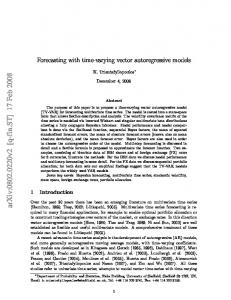
4.4. Forecast Based on the best model of VAR(2) Model, it can be used to obtain forecast values for each region. Data were forecasted for the next 5-year periods. The results of the forecast using the VAR(2) Model for currency outflow data in four regions are as follows: Table 2. Forecasting result with VAR(2) Model Year 2015

Month April May June July August

Semarang 1738.69 1067.71 1208.47 1082.03 969.30

Solo 871.79 506.28 574.30 524.68 464.04

Purwokerto 839.14 448.52 552.15 505.64 441.30

Tegal 510.44 268.24 343.89 309.81 275.71

Plots of the forecasting result are presented below:

Figure 8. Data Plots of the Forecasting Results for the subsequent 5- year periods In Figure 8, the data plot for each region had the same relative data pattern. In this plot, shows the predicted value for Z1 (Outflow of cash in the Representative Office of Bank Indonesia Semarang)

8



was higher compared to 3 other regions. While the forecast value for Z4 (Outflow of cash in the Representative Office of Bank Indonesia Tegal) had the lowest forecast value compared to the other 3 regions. 5. Conclusion According to the results and discussion, the conclusions obtained are as follow: a. The best fit VAR Model for those 4 regions is VAR(2) Model which has the smallest AIC Value and satisfy the white noise assumption. b. The Forecasting results show that the value is fluctuated to the relatively similar data pattern. 6. Suggestions It would be better to do further research, as in addition to the time correlation, it is also region correlation from one region to the others. The next research can be continued with the GSTAR-SUR model approach. References [1] Bank Indonesia. 2006. Perhitungan Uang Kartal yang Diedarkan. Bagian Penelitian dan Pengembangan Pengedaran Uang – DPU. [www.bi.go.id , 12 April 2017]. [2] Borovkova, S.A., Lopuhaa, H.P., and Ruchjana, B.N. 2008. Consistency and asymptotic normality of least square estimators in generalized STAR models. Statistica Neerlandica, Vol. 62, No.4, pp. 482-508. [3] Box, G.E.P., Jenkins, G.M., dan Reinsel, G.C. 1994. Time Series Analysis: Forecasting and Control. 3rd edition, Englewood Cliffs: Prentice Hall. [4] Faizah, L.A. dan Setiawan. 2013. Pemodelan Inflasi di Kota Semarang, Yogyakarta dan Surakarta dengan Pendekatan GSTAR. Jurnal Sains dan Seni Pomits. Vol.2. No.2. pp. 23373520. [5] Gerai Info. 2011. Pengedaran Uang: “Yang Penting Pas Agar Ekonomi Nggak Kolaps”. Sixteenth edition. Jakarta: Bank Indonesia. [6] Lütkepohl, H. 2007. Econometrics Analysis with Vector Autoregressive Models. EUI Working Papers ECO. 1725-6704. [7] Mubarak, R. 2015. Generalized Space-Time Autoregressive with Exogenous Variables Model for Forcasting Cashflow in Bank Indonesia East Java Region. Surabaya: Sepuluh November Institute of Technology. [8] Pramono, B et al. 2006. Dampak Pembayaran Non Tunai Terhadap Perekonomian dan Kebijakan Moneter. Working Paper Nomor 11. Not published. Bank Indonesia. [9] Prayitno, L., Sandjaya, H. dan Llewelyn, R. 2002. Faktor-Faktor Yang Berpengaruh Terhadap Jumlah Uang Beredar di Indonesia Sebelum dan Sesudah Krisis: Sebuah Analisis Ekonometrika. Jurnal Manajemen & Kewirausahaan, Vol. 4, No.1, pp.46–55. [10] Suhartono dan Atok, R.M. 2006. Pemilihan Bobot Lokasi yang Optimal pada model GSTAR. Presented at National Mathematics Conference XIII. Semarang: State University of Semarang. [11] Suhartono dan Subanar. 2006. The Optimal Determination of Space Weight in GSTAR Model by Using Cross-sorrelation Inference. Journal of Quantitative Methods: Journal Devoted the Mathematical and Statistical Application in Various Field. Vol.2. No.2. pp.45-53. [12] Untoro. 2007. Mengkaji Efektivitas Penggunaan ARIMA dan VAR Dalam Melakukan Proyeksi Permintaan Uang Kartal di Indonesia. Buletin Ekonomi Moneter dan Perbankan Buletin Ekonomi Moneter dan Perbankan, Vol.10. No.1, pp. 51-83. [13] Wutsqa, D.U., Suhartono dan Sutijo, B. (2010). Generalized Space-Time Autoregressive Modeling. Proceedings of the 6th IMT-GT Conference on Mathematics, Statistics and its Applications (ICMSA2010), Universiti Tunku Abdul Rahman, Kuala Lumpur, Malaysia, pp. 752-761.

9



[14] Wutsqa, D. U. dan Suhartono. 2010. Seasonal Multivariate Time Series Forecasting on Tourism Data by Using Var-Gstar Model. Jurnal ILMU DASAR, Vol. 11, No. 1, pp. 101-109. [15] Wei, W.W.S. 2006. Time Series Analysis: Univariate and Multivariate Methods. United State of America: Addison-Wesley Publishing Co., USA.

10