all limited to producing prefix classifiers, which means that they all miss the ..... integers whose binary representation matches the ternary string. For purposes of ...
Bit Weaving: A Non-prefix Approach to Compressing Packet Classifiers in TCAMs Chad R. Meiners Alex X. Liu Eric Torng Department of Computer Science and Engineering Michigan State University East Lansing, MI 48823, U.S.A. {meinersc, alexliu, torng}@cse.msu.edu Abstract Ternary Content Addressable Memories (TCAMs) have become the de facto standard in industry for fast packet classification. Unfortunately, TCAMs have limitations of small capacity, high power consumption, high heat generation, and high cost. The well-known range expansion problem exacerbates the problem of smaller TCAMs by significantly decreasing the already limited capacity of these TCAMs as each classifier rule typically has to be converted to multiple TCAM rules. One method for coping with smaller TCAMs is to use compression schemes to reduce the number of TCAM rules required to represent a classifier. Although several TCAM-based classifier compression schemes have been proposed, they are all limited to producing prefix classifiers, which means that they all miss the compression opportunities created by non-prefix ternary classifiers. In this paper, we propose bit weaving, the first nonprefix classifier compression scheme. Bit weaving is based on the observation that adjacent TCAM entries that have a hamming distance of one (i.e., differ by only one bit) can be merged into one entry by replacing the bit in question with *. Bit weaving consists of two new techniques, bit swapping and bit merging, to first identify and then merge such rules together. The key advantages of bit weaving are that it runs fast, and it is composable with other TCAM optimization methods as a pre/postprocessing routine. We implemented bit weaving and conducted experiments on both real-world and synthetic packet classifiers. Our experimental results show the following: (i) bit weaving is an effective stand-alone compression technique (it achieves an average compression ratio of 23.6%) and (ii) bit weaving finds compression opportunities that other methods miss. Specifically, bit weaving improves the prior TCAM optimization techniques of TCAM Razor and Topological Transformation by an average of 12.8% and 36.5%, respectively.
1 Introduction 1.1 Background on TCAM-Based Packet Classification Packet classification is the core mechanism that enables many networking devices, such as routers and firewalls, to perform services such as packet filtering, virtual private networks (VPNs), network address translation (NAT), quality of service (QoS), load balancing, traffic accounting and monitoring, differentiated services (Diffserv), etc. The essential problem is to compare each packet with a list of predefined rules, which we call a packet classifier, and find the first (i.e., highest priority) rule that the packet matches. Table 1 shows an example packet classifier of three rules. The format of these rules is based upon the format used in Access Control Lists (ACLs) on Cisco routers. In this paper we use the terms packet classifiers, ACLs, rule lists, and lookup tables interchangeably. Rule r1 r2 r3
Source IP Dest. IP Source Port Dest. Port Protocol 1.2.3.0/24 192.168.0.1 [1,65534] [1,65534] TCP 1.2.11.0/24 192.168.0.1 [1,65534] [1,65534] TCP * * * * *
Action accept accept discard
Table 1: An example packet classifier Hardware-based packet classification using Ternary Content Addressable Memories (TCAMs) is now the de facto industry standard [1,10]. TCAM-based packet classification is widely used because Internet routers need to classify every packet on the wire. Although software based packet classification has been extensively studied (see survey paper [25]), these techniques cannot match the wire speed performance of TCAM-based packet classification systems. As a traditional random access memory chip receives an address and returns the content of the memory at that address, a TCAM chip works in a reverse manner: it receives content and returns the address of the first entry where the content lies in the TCAM in constant time
(i.e., a few clock cycles). Exploiting this hardware feature, TCAM-based packet classifiers store a rule in each entry as an array of 0’s, 1’s, or *’s (don’t-care values). A packet header (i.e., a search key) matches an entry if and only if their corresponding 0’s and 1’s match. Given a search key to a TCAM, the hardware circuits compare the key with all its occupied entries in parallel and return the index (or the content, depending on the chip architecture and configuration,) of the first matching entry.
their market size [11]. Power consumption, heat generation, board space, and cost lead to system designers using smaller TCAM chips than the largest available. For example, TCAM components are often restricted to at most 10% of an entire board’s power budget, so a 36 Mb TCAM may not be deployable on all routers due to power consumption reasons. While TCAM-based packet classification is the current industry standard, the above limitations imply that existing TCAM-based solutions may not be able to scale up to meet the future packet classification needs of the rapidly growing Internet. Specifically, packet classifiers are growing rapidly in size and width due to several causes. First, the deployment of new Internet services and the rise of new security threats lead to larger and more complex packet classification rule sets. While traditional packet classification rules mostly examine the five standard header fields, new classification applications begin to examine addition fields such as classifierid, protocol flags, ToS (type of service), switch-port numbers, security tags, etc. Second, with the increasing adoption of IPv6, the number of bits required to represent source and destination IP address will grow from 64 to 256. The size and width growth of packet classifiers puts more demand on TCAM capacity, power consumption, and heat dissipation. To address the above TCAM limitations and ensure the scalability of TCAM-based packet classification, we study the following TCAM-based classifier compression problem: given a packet classifier, we want to efficiently generate a semantically equivalent packet classifier that requires fewer TCAM entries. Note that two packet classifiers are (semantically) equivalent if and only if they have the same decision for every packet. TCAM-based classifier compression helps to address the limited capacity of deployed TCAMs because reducing the number of TCAM entries effectively increases the fixed capacity of a chip. Reducing the number of rules in a TCAM directly reduces power consumption and heat generation because the energy consumed by a TCAM grows linearly with the number of ternary rules it stores [28]. Finally, TCAMbased classifier compression lets us use smaller TCAMs, which results in less power consumption, less heat generation, less board space, and lower hardware cost.
1.2 Motivation for TCAM-based Classifier Compression Although TCAM-based packet classification is currently the de facto standard in industry, TCAMs do have several limitations. First, TCAM chips have limited capacity. The largest available TCAM chip has a capacity of 36 megabits (Mb). Smaller TCAM chips are the most popular due to the other limitations of TCAM chips stated below. Second, TCAMs require packet classification rules to be in ternary format. This leads to the well-known range expansion problem, i.e., converting packet classification rules to ternary format results in a much larger number of TCAM rules, which exacerbates the problem of limited capacity TCAMs. In a typical packet classification rule, the three fields of source and destination IP addresses and protocol type are specified as prefixes (e.g., 1011****) where all the *s are at the end of the ternary string, so the fields can be directly stored in a TCAM. However, the remaining two fields of source and destination port numbers are specified in ranges (i.e., integer intervals such as [1, 65534]), which need to be converted to one or more prefixes before being stored in a TCAM. This can lead to a significant increase in the number of TCAM entries needed to encode a rule. For example, 30 prefixes are needed to represent the single range [1, 65534], so 30 × 30 = 900 TCAM entries are required to represent the single rule r1 in Table 1. Third, TCAM chips consume lots of power. The power consumption of a TCAM chip is about 1.85 Watts per Mb [2]. This is roughly 30 times larger than a comparably sized SRAM chip [11]. TCAMs consume lots of power because every memory access searches the entire active memory in parallel. That is, a TCAM is not just memory, but memory and a (very fast) parallel search system. Fourth, TCAMs generate lots of heat due to their high power consumption. Fifth, a TCAM chip occupies a large footprint on a line card. A TCAM chip occupies 6 times (or more) board space than an equivalent capacity SRAM chip [11]. For networking devices such as routers, area efficiency of the circuit board is a critical issue. Finally, TCAMs are expensive, costing hundreds of dollars even in large quantities. TCAM chips often cost more than network processors [12]. The high price of TCAMs is mainly due to their large die area, not
1.3 Limitations of Prior Art Several prior TCAM-based classifier compression schemes (i.e., [3, 6, 7, 14, 18, 24]) have been developed. While these techniques vary in effectiveness, they all suffer from one fundamental limitation: they only produce prefix classifiers, which means they all miss some opportunities for compression. A prefix classifier is a classifier in which every rule is a prefix rule. A prefix rule is a rule in which each field is specified as a prefix bit string (e.g., 2
F1 F2 Partition 1 Partition 2
00 10 0* 0* **
0* 0* 00 10 **
Swap
F1 F2
1 1 Bit 2swapping 2 0
000* 1 100* 1 000* 2 001* 2 **** 0
Minimizing
000* 1 100* 1 00** 2 **** 0
*00* 1 Bit Recovery
Bit Merging
00** 2 **** 0
*0 0* 1 0* *0 2 ** ** 0
Figure 1: Example of the bit weaving approach 01**), where *s all appear at the end. A ternary rule is a rule in which each field is a ternary bit string (e.g., 0**1), where * can appear at any position. Clearly, every prefix rule is a ternary rule, but not vice versa. Because all previous compression schemes can only produce prefix rules while TCAMs only require that every rule be a ternary rule, all previous compression schemes miss the compressiob opportunities created by non-prefix ternary rules.
partition requires no bit swapping because it is already a list of one-dimensional prefix rules. For the second partition, it swaps the second and the fourth columns. We call the above two steps bit swapping. Third, we treat each partition as a one-dimensional prefix rule list and minimize each partition to its minimal prefix representation. In this example, the second partition is minimized to 2 rules. Fourth, in each partition, we detect and merge rules that differ by a single bit. We call this step bit merging. Finally, we revert each partition back to its original bit order. In this example, for the second partition after minimization, we swap the second and the fourth columns again to recover the original bit order. The final output is a ternary packet classifier with only 3 rules.
1.4 Our Bit Weaving Approach In this paper, we propose bit weaving, a new TCAMbased classifier compression scheme that is not limited to producing prefix classifiers. The basic idea of bit weaving is simple: adjacent TCAM entries that have a hamming distance of one (i.e., differ by only one bit) can be merged into one entry by replacing the bit in question with *. Bit weaving applies two new techniques, bit swapping and bit merging, to first identify and then merge such rules together. Bit swapping first cuts a rule list into a series of partitions. Within each partition, a single permutation is applied to each rule’s predicate to produce a reordered rule predicate, which forms a single prefix where all *’s are at the end of the rule predicate. This single prefix format allows us to use existing dynamic programming techniques [18,24] to find a minimal TCAM table for each partition in polynomial time. Bit merging then searches each partition and merges together rules that differ by a single bit. Once both techniques are finished, we revert all ternary strings back to their original bit permutation to produce the final TCAM table. We name our solution bit weaving because it manipulates bit ordering in a ternary string much like a weaver manipulates the position of threads. The example in Figure 1 shows that our bit weaving approach can further compress a minimal prefix classifier. The input classifier has 5 prefix rules with three decisions (0, 1, and 2) over two fields F1 and F2 , where each field has two bits. Our bit weaving approach compresses this minimal prefix classifier with 5 rules down to 3 ternary rules as follows. First, it cuts the input prefix classifier into two partitions; the first partition consists of the first 2 rules, and the second partition consists the remaining 3 rules. Second, it treats each partition as a one-dimensional ternary rule list and swaps bit columns in each partition to make each partition a list of one-dimensional prefix rules. In this example, the first
1.5 Technical Challenges To implement bit weaving, we must solve several challenging technical problems. First, we must develop an algorithm that partitions a rule list into a minimal number of partitions. Second, we must develop an algorithm that permutes the bit columns within each partition to produce one-dimensional prefix rule lists. Third, we must adapt existing one-dimensional prefix rule list minimization algorithms (i.e., [18, 24]) to minimize incomplete one-dimensional rule lists. A rule list is complete if and only if for any packet, the list has a rule that the packet matches. Finally, we must develop algorithms to detect and then merge mergeable rules within each partition. Although it is obvious that two adjacent rules with one bit difference can be merged, it is less obvious how we can find other mergeable rules.
1.6 Our Contributions Our bit weaving approach has many significant benefits. First, it is the first TCAM compression method that can create non-prefix classifiers. All previous compression methods [6, 13, 15, 18] generate only prefix classifiers. This restriction to prefix format may miss important compression opportunities. Second, it is the first efficient compression method with a polynomial worst-case running time with respect to the number of fields in each rule. Third, it is orthogonal to other techniques, which means that it can be run as a pre/post-processing routine in combination with other compression techniques. In particular, bit weaving complements TCAM Razor [18] nicely. In our experiments on real-world classifiers, bit 3
weaving achieves higher compression ratios on the classifiers that TCAM Razor has lower compression ratios. Fourth, it supports fast incremental updates to classifiers.
finds locally minimal prefix solutions along each field and combines these solutions into a smaller equivalent prefix packet classifier [18]. Bit weaving differs from these previous efforts in that it is the first classifier minimization algorithm that produces equivalent non-prefix packet classifiers given an arbitrary number of fields and decisions. Furthermore, bit weaving is the first algorithm whose worst-case running time is polynomial with respect to the number of fields within a classifier.
1.7 Summary of Experimental Results We implemented bit weaving and conducted experiments on both real-world and synthetic packet classifiers. Our experimental results show that bit weaving is an effective stand-alone compression technique as it achieves an average compression ratio of 23.6% and that bit weaving finds compression opportunities that other methods miss. Specifically, bit weaving improves the prior TCAM optimization techniques of TCAM Razor [18], and Topological Transformation [20] by an average of 12.8% and 36.5%, respectively. The rest of this paper proceeds as follows. We start by reviewing related work in Section 2 and defining concepts and notation in Section 3. We define bit swapping in Section 4 and bit merging in Section 5. In Section 6, we discuss how bit weaving supports incremental updates, how bit weaving can be composed with other compression methods, and the complexity bounds of bit weaving. We show our experimental results on both reallife and synthetic packet classifiers in Section 7, and we give concluding remarks in Section 8.
2.2 Range Encoding Range encoding schemes cope with range expansion by developing a new representation for important packets and intervals. For example, a new representation for interval [1, 65534] may be developed so that this interval can be represented with one TCAM entry rather than 900 prefix entries. Previous range encoding schemes fall into two categories: database independent encoding schemes [4, 10], where each rule is encoded according to standard encoding scheme, and database dependent encoding schemes [5, 16, 20, 21, 27], where the encoding of each rule depends the intervals present within the classifier. While range encoding methods do mitigate the effects of prefix expansion, they require either extra hardware or more per packet processing time.
2 Related Work TCAM-based packet classification systems have been widely deployed due to their O(1) classification time. This has led to a significant amount of work that explores ways to efficiently store packet classifiers within TCAMs. Prior work falls into three broad categories: classifier compression, range encoding, and circuit and hardware modification.
2.3 Circuit and Hardware Modification These techniques modify TCAM circuits to accommodate range comparisons. For example, Spitznagel et al. proposed adding comparators at each entry level to better accommodate range matching [23]. While this research direction is important, our contribution does not require circuit-level modifications to hardware. Additionally, there has been work on developing load balancing algorithms for TCAM based systems by Zheng et al. [29,30]. This work focuses on exploiting chip level parallelism to increase classifier throughput with multiple TCAM chips without having to copy the complete classifier to every TCAM chip. This work may benefit from bit weaving since fewer rules would need to be distributed among the TCAM chips. From a different perspective, [19] proposed a multiple TCAM chip architecture that reduces a multiple field classifier into a series of single field classifiers.
2.1 Classifier Compression Classifier compression converts a given packet classifier to another semantically equivalent packet classifier that requires fewer TCAM entries. Several classifier compression schemes have been proposed [3, 6, 7, 13, 18, 24]. The work is either focused on one-dimensional and two dimensional packet classifiers [3, 7, 24], or it is focused on compressing packet classifiers with more than 2 dimensions [6, 13, 15, 18]. Liu and Gouda proposed the first algorithm for eliminating all the redundant rules in a packet classifier [13], and we presented a more efficient redundancy removal algorithm [15]. Dong et al. proposed schemes to reduce range expansion by repeatedly expanding or trimming ranges to prefix boundaries [6]. Their schemes use redundancy removal algorithms [13] to test whether each modification changes the semantics of the classifier. We proposed a greedy algorithm that
3 Background We now formally define the concepts of fields, packets, and packet classifiers. A field Fi is a variable of finite length (i.e., of a finite number of bits). The domain of field Fi of w bits, denoted D(Fi ), is [0, 2w −1]. A packet over the d fields F1 , · · · , Fd is a d-tuple (p1 , · · · , pd ) 4
where each pi (1 ≤ i ≤ d) is an element of D(Fi ). Packet classifiers usually check the following five fields: source IP address, destination IP address, source port number, destination port number, and protocol type. The lengths of these packet fields are 32, 32, 16, 16, and 8, respectively. We use Σ to denote the set of all packets over fields F1 , · · · , Fd . It follows that Σ is a finite set and |Σ| = |D(F1 )| × · · · × |D(Fd )|, where |Σ| denotes the number of elements in set Σ and |D(Fi )| denotes the number of elements in set D(Fi ). A rule has the form hpredicatei → hdecisioni. A hpredicatei defines a set of packets over the fields F1 through Fd , and is specified as F1 ∈ S1 ∧ · · · ∧ Fd ∈ Sd where each Si is a subset of D(Fi ) and is specified as either a ternary string, a prefix or a nonnegative integer interval. A ternary string {0, 1, ∗}k denotes the set of integers whose binary representation matches the ternary string. For purposes of matching, the ∗ is treated as a wild card. For example, the string ∗0 denotes the set {0, 2}. A prefix {0, 1}k {∗}w−k with k leading 0s or 1s for a packet field of length w denotes the integer interval [{0, 1}k {0}w−k , {0, 1}k {1}w−k ] and is a special case of a ternary string. For example, prefix 01** denotes the interval [0100, 0111]. A rule F1 ∈ S1 ∧ · · · ∧ Fd ∈ Sd → hdecisioni is a prefix rule if and only if each Si is a prefix, and a rule is a ternary rule if and only if each Si is a ternary string. Every prefix rule is a ternary rule, but not vice versa. A packet matches a rule if and only if the packet matches the predicate of the rule. A packet (p1 , · · · , pd ) matches a predicate F1 ∈ S1 ∧ · · · ∧ Fd ∈ Sd if and only if the condition p1 ∈ S1 ∧ · · · ∧ pd ∈ Sd holds. We use DS to denote the set of possible values that hdecisioni can be. Typical elements of DS include accept, discard, accept with logging, and discard with logging. A sequence of rules hr1 , · · · , rn i is complete if and only if for any packet p, there is at least one rule in the sequence that p matches. To ensure that a sequence of rules is complete and thus a packet classifier, the predicate of the last rule is usually specified as F1 ∈ D(F1 )∧· · · Fd ∈ ∧D(Fd ). A packet classifier C is a sequence of rules that is complete. The size of C, denoted |C|, is the number of rules in C. A packet classifier C is a prefix packet classifier if and only if every rule in C is a prefix rule, and a packet classifier C is a ternary packet classifier if and only if every rule in C is a ternary rule. Every prefix classifier is a ternary classifier, but not vice versa. Two rules in a packet classifier may overlap; that is, a single packet may match both rules. Furthermore, two rules in a packet classifier may conflict; that is, the two rules not only overlap but also have different decisions. Packet classifiers typically resolve such conflicts by employing a first-match resolution strategy where the decision for a packet p is the decision of the first (i.e., high-
est priority) rule that p matches in C. The decision that packet classifier C makes for packet p is denoted C(p). We can think of a packet classifier C as defining a many-to-one mapping function from Σ to DS. Two packet classifiers C1 and C2 are equivalent, denoted C1 ≡ C2 , if and only if they define the same mapping function from Σ to DS; that is, for any packet p ∈ Σ, we have C1 (p) = C2 (p). For any classifier C, we denote the set of equivalent classifiers as {C}. A rule is redundant in a classifier if and only if removing the rule does not change the semantics of the classifier. In a typical packet classifier rule, the fields of source IP, destination IP, and protocol type are specified in prefix format, which can be directly stored in TCAMs; however, the remaining two fields of source port and destination port are specified as ranges (i.e., non-negative integer intervals), which are typically converted to prefixes before being stored in TCAMs. This leads to range expansion, the process of converting a non-prefix rule to prefix rules. In range expansion, each field of a rule is first expanded separately. The goal is to find a minimum set of prefixes such that the union of the prefixes corresponds to the range. For example, if one 3-bit field of a rule is the range [1, 6], a corresponding minimum set of prefixes would be 001, 01∗, 10∗, 110. The worst-case range expansion of a w−bit range results in a set containing 2w − 2 prefixes [8]. The next step is to compute the cross product of the set of prefixes for each field, resulting in a potentially large number of prefix rules.
4 Bit Swapping In this section, we present a new technique called bit swapping. It is the first part of our bit weaving approach.
4.1 Prefix Bit Swapping Algorithm Definition 4.1 (Bit-swap). A bit-swap β of a length m ternary string t is a permutation of the m ternary bits; that is, β rearranges the order of the ternary bits of t. The resulting permuted ternary string is denoted β(t). 2 For example, if β is permutation 312 and string t is 0∗1, then β(t) = 10∗. For any length m string, there are m! different permutations and thus m! different bitswaps. A bit-swap β of a ternary string t is a prefix bitswap if the permuted string β(t) is in prefix format. Let P (t) denote the set of prefix bit-swaps for ternary string t: specifically, the bit-swaps that move the ∗ bits of t to the end of the string. A bit-swap β can be applied to a list ℓ of ternary strings ht1 , . . . , tn i where ℓ is typically a list of consecutive rules in a packet classifier. The resulting list of permuted strings is denoted as β(ℓ). Bit-swap β is a prefix bit-swap for ℓ if β is a prefix bit-swap for every string ti 5
in list ℓ for 1 ≤ i ≤ n. Let P (ℓ) denote the set of prefix bit-swaps for list ℓ. It follows that P (ℓ) = ∩ni=1 P (ti ). Prefix bit-swaps are useful for compressing classifiers for two main reasons. First, we can minimize prefix rule lists using algorithms in [7, 18, 24]. Second, prefix format facilitates the second key idea of bit weaving, bit merging (Section 5). After compressing the bit-swapped classifier, the classifier is reverted to its original bit order, which typically results in a non-prefix format classifier. Unfortunately, given a list ℓ of ternary strings, it is possible that P (ℓ) = ∅, which means that no bit-swap is a prefix bit-swap for every string in ℓ. For example, the list h0∗, ∗0i does not have a valid prefix bit-swap. A natural question to ask is what are the necessary and sufficient conditions for P (ℓ) = ∅. Given that each ternary string denotes a set of binary strings, we define two new operators for ternary strings: ˆ0(x) and ⊑. For any ternary string x, ˆ0(x) denotes the resulting ternary string where every 1 in x is replaced by 0. For example, ˆ0(1*)=0*. For any two ternary strings x and y, x ⊑ y if and only if ˆ0(x) ⊆ ˆ0(y). For example, 1*⊑0* because ˆ0(1*)=0*={00, 01} ⊆ {00, 01}=ˆ0(0*).
Figure 2: Example of bit-swapping Theorem 4.1 gives us a simple algorithm for detecting whether a prefix bit-swap exists for a list of ternary strings. If a prefix bit-swap exists, the proof of Theorem 4.1 gives us a simple and elegant algorithm for constructing a prefix bit-swap as shown in Algorithm 1. The algorithm sorts bit columns in an increasing order by the number of strings that have a ∗ in that column. Before we formally present our bit swapping algorithm, we define the concepts of bit matrix and decision array for a possibly incomplete rule list (i.e., there may exist at least one packet that none of the n rules matches). Any list of n rules defines a bit matrix M [1..n, 1..b] and a decision array D[1..n], where for any 1 ≤ i ≤ n and 1 ≤ j ≤ b, M [i, j] is the j-th bit in the predicate of the i-th rule and D[i] is the decision of the i-th rule. Conversely, a bit matrix M [1..n, 1..b] and a decision array D[1..n] also uniquely defines a rule list. Given a bit matrix M [0..n − 1, 0..b − 1] and a decision array D[1..n] defined by a rule list, our bit swapping algorithm swaps the columns in M such that for any two columns i and j in the resulting bit matrix M ′ where i < j, the number of *s in the i-th column is less than or equal to the number of *s in the j-th column. Figure 2(a) shows a bit matrix and Figure 2(b) shows the resulting bit matrix after bit swapping. Let L1 denote the rule list defined by M and D, and let L2 denote the rule list defined by M ′ and D. Usually, L1 will not be equivalent to L2 . This is not an issue. The key is that if we revert the bit-swap on any rule list L3 that is equivalent to L2 , the resulting rule list L4 will be equivalent to L1 .
Definition 4.2 (Cross Pattern). Given two ternary strings t1 and t2 , a cross pattern on t1 and t2 exists if and only if (t1 6⊑ t2 ) ∧ (t2 6⊑ t1 ). In such cases, we say that t1 crosses t2 . 2 We first observe that bit swaps have no effect on whether or not two strings cross each other. Observation 4.1. Given two ternary strings, t1 and t2 , and a bit-swap β, t1 ⊆ t2 if and only if β(t1 ) ⊆ β(t2 ), and t1 ⊑ t2 if and only if β(t1 ) ⊑ β(t2 ). 2 Theorem 4.1. Given a list ℓ = ht1 , . . . , tn i of n ternary strings, P (ℓ) 6= ∅ if and only if no two ternary strings ti and tj (1 ≤ i < j ≤ n) cross each other. 2 Proof. (implication) It is given that there exists a prefix bit-swap β ∈ P (ℓ). Suppose that string ti crosses string tj . According to Observation 4.1, β(ti ) crosses β(tj ). This implies that one of the two ternary strings β(ti ) and β(tj ) has a ∗ before a 0 or 1 and henceforth is not in prefix format. Thus, β is not in P (ℓ), which is a contradiction. (converse) It is given that no two ternary strings cross each other. It follows that we can impose a total order on the ternary strings in ℓ using the relation ⊑. Note, there may be more than one total order if ti ⊑ tj and tj ⊑ ti for some values of i and j. Let us reorder the ternary strings in ℓ according to this total order; that is, t′1 ⊑ t′2 ⊑ · · · ⊑ t′n−1 ⊑ t′n . Any bit swap that puts the ∗ bit positions of t′1 last, preceded by the ∗ bit positions of t′2 , . . . , preceded by the ∗ bit positions of t′n , finally preceded by all the remaining bit positions will be a prefix bit-swap for ℓ. Thus, the result follows.
4.2 Minimal Cross-Free Classifier Partitioning Algorithm Given a classifier C, if P (C) = ∅, we cut C into partitions where each partition has no cross patterns and thus has a prefix bit-swap. We treat classifier C as a list of ternary strings by ignoring the decision of each rule. Given an n-rule classifier C = hr1 , . . . , rn i, a partition P on C is a list of consecutive rules hri , . . . , rj i in C for some i and j such that 1 ≤ i ≤ j ≤ n. A partitioning, P1 , . . . , Pk , of C is a series of k partitions on C such that the concatenation of P1 , . . . , Pk is C. A partitioning is cross-free if and only if each partition has no cross patterns. Given a classifier C, a cross-free partitioning with k partitions is minimal if and only if any partitioning of C with k − 1 partitions is not cross-free. 6
F1
F2
** 100000 ** 100010 ** 100100 ** 100110 ** 101000 ** 110000 ** 111000
1 1 1 1 1 1 1
01 ****** 2 1* ****** 2 ** ****** 0
100000** 100010** 100100** 100110** 101000** 110000** 111000**
Bit swapping
1 1 1 1 1 1 1
100000** 100010** 100100** 100110** 101000** 110000** 111000**
Minimizing
01****** 2 1******* 2 ******** 0
1 1 1 1 1 1 1
00****** 0 ******** 2
100**0** 1 1**000** 1 Bit Merging
**100**0 1 **1**000 1 Bit Recovery
00****** 0 ******** 2
00****** 0 ******** 2
Figure 3: Applying bit weaving algorithm to an example classifier imal cross-free partitioning for a given classifier. At any time, we have one active partition. The initial active partition is the last rule of the classifier. We consider each rule in the classifier in reverse order and attempt to add it to the active partition. If the current rule crosses any rule in the active partition, that partition is completed, and the active partition is reset to contain only the new rule. It is not hard to prove that this algorithm produces a minimal cross-free partitioning for any given classifier. The core operation in the above cross-free partitioning algorithm is to check whether two ternary strings cross each other. We next present Theorem 4.2, which gives us an efficient algorithm for performing such checking. For any ternary string t of length m, we define the bit mask of t, denoted M (t), to be a binary string of length m where the i-th bit (0 ≤ i < m) M (t)[i] = 0 if t[i] = ∗ and M (t)[i] = 1 otherwise. For any two binary strings a and b, we use a && b to denote the resulting binary string of the bitwise logical AND of a and b.
Algorithm 1: Finds a prefix bit-swap Input: A classifier C with n rules r1 , . . . , rn where each rule has b bits. Output: A classifier C ′ that is C after a valid prefix bit-swap.
7
Let M [1 . . . n, 1 . . . b] and D[1 . . . n] be the bit matrix and decision array of C; Let B = h(i, j)|1 ≤ i ≤ n and j is the number of *’s in M [1 . . . n, i]i; Sort B in ascending order of each pair’s second value; Let M ′ be a copy of M ; for k := 1 to b do Let (i, j) = B[k]; M ′ [1 . . . n, k] := M [1 . . . n, i];
8
Output C ′ defined by M ′ and D;
1 2 3 4 5 6
The goal of classifier partitioning is to find a minimal cross-free partitioning for a given classifier. We then apply independent prefix bit-swaps to each partition. After bit-swapping each partition, we compress each partition using the optimal prefix minimization algorithm in [18] followed by bit merging (Section 5). Then, we revert each bit-swapped partition to recover the original order of each column, which yields non-prefix rules. Finally, the concatenation of each resulting partition constitutes the final compressed non-prefix field classifier.
Theorem 4.2. For any two ternary string t1 and t2 , t1 does not cross t2 if and only if M (t1 ) && M (t2 ) is equal to M (t1 ) or M (t2 ). 2 For example, given two ternary strings t1 = 01∗0 and t2 = 101∗, whose bit masks are M (t1 ) = 1101 M (t1 ) = 1110, we have M (t1 ) && M (t2 ) = 1100. Therefore, t1 = 01∗0 crosses t2 = 101∗ because M (t1 ) && M (t2 ) 6= M (t1 ) and M (t1 ) && M (t2 ) 6= M (t2 ). Figure 3 shows the execution of our bit weaving algorithm on an example classifier. Here we describe the bit swapping portion of that execution. The input classifier has 10 prefix rules with three decisions (0, 1, and 2) over two fields F1 and F2 , where F1 has two bits, and F2 has six bits. We begin by constructing a maximal cross-free partitioning of the classifier by starting at the last rule and working upward. We find that the seventh rule introduces a cross pattern with the eighth rule according to Theorem 4.2. This results in splitting the classifier into two partitions. Second, we perform bit swapping on each partition, which converts each partition into a list of onedimensional prefix rules.
Algorithm 2: Find a minimal partition Input: A list of n rules hr1 , . . . , rn i each rule has b bits. Output: A list of partitions.
6
Let P be the current partition (empty list), and L be a list of partitions (empty); for i := n to 1 do if ri introduces a cross pattern in P then Append P to the head of L; else Append ri to the head of P ;
7
return L;
1 2 3 4 5
To maximize bit weaving’s effectiveness, we develop an algorithm, depicted in Algorithm 2, that finds a min7
4.3 Partial List Minimization Algorithm
5 Bit Merging In this section, we present bit merging, the second part of our bit weaving approach. The fundamental idea behind bit merging is to repeatedly find in a classifier two ternary strings that differ only in one bit and replace them with a single ternary string where the differing bit is ∗.
We now describe how to minimize each bit swapped partition where we view each partition as a list of 1dimensional prefix rules. If a list of 1-dimensional prefix rules is complete (i.e., any packet has a matching rule in the list), we can use the algorithms in [7, 24] to produce an equivalent minimal prefix rule list. However, the rule list in a partition is often incomplete; that is, there exist packets that do not match any rule in the partition. In this paper, we adapt the Weighted 1-Dimensional Prefix List Minimization Algorithm in [18] to solve this problem of minimizing incomplete or partial rule lists. Given a 1-dimensional packet classifier f of n prefix rules hr1 , r2 , · · · , rn i, where {Decision(r1 ), Decision(r2 ), · · · , Decision(rn )} = {d1 , d2 , · · · , dz } and each decision di is associated with a cost Cost (di ) (for 1 ≤ i ≤ z), the cost of packet classifier f is defined as follows [18]: Cost (f ) = Pn i=1 Cost (Decision(ri )). The problem of weighted one-dimensional TCAM minimization is stated as follows [18]: Given a one-dimensional packet classifier f1 where each decision is associated with a cost, find a prefix packet classifier f2 ∈ {f1 } such that for any prefix packet classifier f ∈ {f1 }, the condition Cost (f2 ) ≤ Cost (f ) holds.
5.1 Definitions When two ternary strings t1 and t2 differ only in one bit, i.e., their hamming distance [9] is one, and we say the two strings are ternary adjacent. The ternary string produced by replacing the one differing bit by a ∗ in t1 (or t2 ) is called the ternary cover of t1 and t2 . For example, 0∗∗ is the ternary cover for 00∗ and 01∗. We call the process of replacing two ternary adjacent strings by their cover bit merging or just merging. For example, we can merge 00∗ and 01∗ to form their cover 0∗∗. We now define how to bit merge (or just merge) two rules. For any rule r, we use P(r) to denote the predicate of r. Two rules ri and rj are ternary adjacent if their predicates P(ri ) and P(rj ) are ternary adjacent. The merger of ternary adjacent rules ri and rj is a rule whose predicate is the ternary cover of P(ri ) and P(rj ) and whose decision is the decision of rule ri . We give a necessary and sufficient condition where bit merging two rules does not change the semantics of a classifier.
We adapt the Weighted 1-Dimensional Prefix List Minimization Algorithm in [18] to minimize a partial 1dimensional prefix rule list L over field F as follows. Let {d1 , d2 , · · · , dz } be the set of all the decisions of the rules in L. Let L denote the list of prefix rules that is the complement of L (i.e., any packet has one matching rule in either L or L, but not both) and each rule in L is assigned the same decision dz+1 that is not in {d1 , d2 , · · · , dz }). First, we assign each decision in {d1 , d2 , · · · , dz } a weight of 1 and the decision dz+1 a weight of |D(F )|, the size of the domain F . Second, we concatenate L with L to form a complete prefix classifier L′ , and run the weighted 1-dimensional prefix list minimization algorithm in [18] on L′ . Since this algorithm outputs a prefix classifier whose sum of the decision weights is the minimum, our weight assignment guarantees that decision dz+1 only appears in the last rule in the minimized prefix classifier. Let L′′ be the resulting minimized prefix classifier. Finally, we remove the last rule from L′′ . The resulting prefix list is the minimal prefix list that is equivalent to L.
Theorem 5.1. Any two rules in a classifier can be merged into one rule without changing the classifier semantics if and only if they satisfy the following three conditions: (1) they can be moved to be adjacent without changing the semantics of the classifier; (2) they are ternary adjacent; (3) they have the same decision (in order to preserve the semantics of the classifier). 2 The basic idea of bit merging is to repeatedly find two rules in the same bit-swapped partition that can be merged based on the three conditions in Theorem 5.1. We do not consider merging rules from different bitswapped partitions because any two bits from the same column in the two bit-swapped rules may correspond to different columns in the original rules.
5.2 Bit Merging Algorithm (BMA) 5.2.1 Prefix Chunking To address the first condition in Theorem 5.1, we need to quickly determine what rules in a bit-swapped partition can be moved together without changing the semantics of the partition (or classifier). For any 1-dimensional minimum prefix classifier C, let Cs denote the prefix classifier formed by sorting all the rules in C in decreasing order of prefix length. We prove that C ≡ Cs if C is a 1-dimensional minimum prefix classifier in Theorem 5.2.
Continuing the example from Figure 3, we use the partial prefix list minimization algorithm to minimize each partition to its minimal prefix representation. In this example, this step eliminates one rule from the bottom partition. 8
5.2.3 Algorithm and Optimality
Before we introduce and prove Theorem 5.2, we first present Lemma 5.1. Note that a rule r is upward redundant if and only if there are no packets whose first matching rule is r [13]. Clearly, upward redundant rules can be removed from a classifier with no change in semantics.
The bit merging algorithm (BMA) works as follows. BMA takes as input a minimum, possibly incomplete prefix classifier C that corresponds to a cross-free partition generated by bit swapping. BMA first creates classifier Cs by sorting the rules of C in decreasing order of their prefix length and partitions Cs into prefix chunks. Second, for each prefix chunk, BMA groups all the rules with the same bit mask and decision together, eliminates duplicate rules, and searches within each group for mergeable rules. The second step repeats until no group contains rules that can be merged. Let C′ denote the output of the algorithm. Figure 4 demonstrates how BMA works. On the leftmost side is the first partition from Figure 3. On the first pass, eight ternary rules are generated from the original seven. For example, the top two rules produce the rule 1000*0** → 1. These eight rules are grouped into four groups with identical bit masks. On the second pass, two unique rules are produced by merging rules from the four groups. Since each rule is in a separate group, no further merges are possible and the algorithm finishes. Algorithm 3 shows the general algorithm for BMA.
Lemma 5.1. For any two rules ri and rj (i < j) in a prefix classifier hr1 , · · · , rn i that has no upward redundant rules, P(ri ) ∩ P(rj ) 6= ∅ if and only if P(ri ) ⊂ P(rj ). 2 Theorem 5.2. For any one-dimensional minimum prefix packet classifier C, we have C ≡ Cs . 2 Proof. Consider any two rules ri , rj (i < j) in C. If the prefixes of ri and rj do not overlap (i.e., P(ri ) ∩ P(rj ) = ∅), changing the relative order between ri and rj does not change the semantics of C. If the prefixes of ri and rj do overlap (i.e., P(ri ) ∩ P(rj ) 6= ∅), then according to Lemma 5.1, we have P(ri ) ⊂ P(rj ). This means that P(ri ) is strictly longer than P(rj ). This implies that ri is also listed before rj in Cs . Thus, the result follows. Based on Theorem 5.2, given a minimum sized prefix bit-swapped partition, we first sort the rules in decreasing order of their prefix length. Second, we further partition the rules into groups based on their prefix length; we call these groups prefix chunks. According to Theorem 5.2, the order of the rules in each prefix chunk is irrelevant, so the rules can be reordered without changing the semantics of the partition.
Figure 4: Example of Bit Merging Algorithm Execution 5.2.2 Bit-Mask Grouping Algorithm 3: Bit Merging Algorithm To address the second condition in Theorem 5.1, we need to quickly determine what rules are ternary adjacent. Based on Theorem 5.3, we can significantly reduce our search space by searching for mergeable rules only among the rules which have the same bit mask and decision.
Input: A list I of n rules hr1 , . . . , rn i where each rule has b bits. Output: A list of m rules. 1 2
Theorem 5.3. Given a list of rules where the rules have the same decision and no rule’s predicate is a proper subset of another rule’s predicate, if two rules are mergeable, then the bit masks of their predicates are the same.
3 4 5 6 7
Proof. Suppose in such a list there are two rules ri and rj that are mergeable and have different bit masks. Because they are mergeable, P(ri ) and P(rj ) differ in only one bit. Because the bit masks are different, one predicate must have a ∗ and the other predicate must have a 0 or 1 in that bit column. Without loss of generality, let ri be the rule whose predicate has a ∗. Because the two rules have the same decision, P(rj ) ⊂ P(ri ), which is a contradiction.
8 9 10 11 12
9
Let S be the set of rules in I; Let C be the partition of S such that each partition contains a maximal set of rules in S such each rule has an identical bitmask and decision; Let OS be an empty set; ′ for each c = {r1′ , . . . , rm } ∈ C do for i := 1 to m − 1 do for j := i + 1 to m do if P(ri′ ) and P(rj′ ) are ternary adjacent then Add the ternary cover of P(ri′ ) and P(rj′ ) to OS; Let O be OS sorted in decreasing order of their prefix length; if S = OS then return O; else return the result of BMA with O as input;
The correctness of this algorithm, C′ ≡ C, is guaranteed because we only combine mergeable rules. We now prove that BMA is locally optimal as stated in Theorem 5.4.
6.2 Incremental Classifier Updates Classifier rules periodically need to be updated when networking services change. Sometimes classifiers are updated manually by network administrators, in which case the timing is not a concern and rerunning the fast bit weaving algorithm will suffice. Sometimes classifiers are updated automatically in an incremental fashion; in these cases, fast updates may be critically important. Our bit weaving approach supports efficient incremental classifier changes by confining change impact to one cross-free partition. An incremental classifier change is typically one of the three actions: inserting a new rule, deleting an existing rule, or modifying a rule. Given a change, we first locate the cross-free partition where the change occurs by consulting a precomputed list of all the rules in each partition. Then we rerun the bit weaving algorithm on the affected partition. We may need to further divide the partition into cross-free partitions if the change introduces a cross pattern. Note that deleting a rule never introduces cross patterns. The experimental data used in Section 7 indicates that only 2.7% of partitions have more than 32 rules and 0.6% of partitions have more than 128 rules for real life classifiers. For synthetic classifiers, these percentages are 17.3% and 0.9%, respectively. For these classifiers, incremental classifier updates are fast and efficient. To further evaluate the incremental update times, we divided each classifier into a top half and a bottom half. We constructed a classifier for the bottom half and then incrementally added each rule from the top half classifier. Using this test, we found that incrementally adding a single rule takes on average 2ms with a standard deviation of 4ms for real world classifiers, and 6ms with a standard deviation of 5ms for synthetically generated classifiers.
Lemma 5.2. During each execution of the second step, BMA never introduces two rules ri and rj such that P(ri ) ⊂ P(rj ) where both ri and rj have the same decision. 2 Lemma 5.3. Consider any prefix chunk in Cs . Let k be the length of the prefix of this prefix chunk. Consider any rule r in C′ that was formed from this prefix chunk. The kth bit of r must be 0 or 1, not ∗. 2 Theorem 5.4. The output of BMA, C′ , contains no pair of mergeable rules. Proof. Within each prefix chunk, after applying BMA, there are no pairs of mergeable rules for two reasons. First, by Theorem 5.3 and Lemma 5.2, in each run of the second step of the algorithm, all mergeable rules are merged. Second, repeatedly applying the second step of the algorithm guarantees that there are no mergeable rules in the end. We now prove that any two rules from different prefix chunks cannot be merged. Let ri and rj be two rules from two different prefix chunks in C′ with the same decision. Suppose ri is from the prefix chunk of length ki and rj is from the prefix chunk of length kj where ki > kj . By Lemma 5.3, the ki -th bit of ri ’s predicate must be 0 or 1. Because ki > kj , the ki -th bit of rj ’s predicate must be ∗. Thus, if ri and rj are mergeable, then ri and rj should only differ in the ki -th bit of their predicates, which means P(ri ) ⊂ P(rj ). This conflicts with Lemma 5.2.
6.3 Composability of Bit Weaving Bit weaving, like redundancy removal, never returns a classifier that is larger than its input. Thus, bit weaving, like redundancy removal, can be composed with other classifier minimization schemes. Since bit weaving is an efficient algorithm, we can apply it as a postprocessing step with little performance penalty. As bit weaving uses techniques that are significantly different than other compression techniques, it can often provide additional compression. We can also enhance other compression techniques by using bit weaving, in particular bit merging, within them. Specifically, multiple techniques [5,18–21] rely on generating single field TCAM tables. These approaches generate minimal prefix tables, but minimal prefix tables can be further compressed by applying bit merging. Therefore, every such technique can be enhanced with bit merging (or more generally bit weaving). For example, TCAM Razor compresses multiple field classifiers by converting a classifier into multiple single
Continuing the example in Figure 3, we perform bit merging on both partitions to reduce the first partition to two rules. Finally, we revert each partition back to its original bit order. After reverting each partition’s bit order, we recover the complete classifier by appending the partitions together. In Figure 3, the final classifier has four rules.
6 Discussion 6.1 Redundancy Removal Our bit weaving algorithm uses the redundancy removal procedure [13] as both the preprocessing and postprocessing step. We apply redundancy removal at the beginning because redundant rules may introduce more cross patterns. We apply redundancy removal at the end because our incomplete 1-dimensional prefix list minimization algorithm may introduce redundant rules across different partitions. 10
of A′ over A assesses how much additional compression is achieved when adding A′ to A.
field classifiers, finding the minimal prefix classifiers for these classifiers, and then constructing a new prefix field classifier from the prefix lists. A natural enhancement is to use bit merging to convert the minimal prefix rule lists into smaller non-prefix rule lists. In our experiments, bit weaving enhanced TCAM Razor [18] yields significantly better compression results than TCAM Razor alone. Range encoding techniques [5, 16, 20, 21, 27] can also be enhanced by bit merging. Range encoding techniques require lookup tables to encode fields of incoming packets. When such tables are stored in TCAM, they are stored as single field classifiers. Bit merging offers a low cost method to further compress these lookup tables. Our results show that bit merging significantly compresses the lookup tables formed by the topological transformation technique [20].
Compression Ratio Average Total |A(C)| ΣC∈S |Direct(C)| |S|
ΣC∈S |A(C)| ΣC∈S |Direct(C)|
Expansion Ratio Average Total ΣC∈S |A(C)| |C| |S|
ΣC∈S |A(C)| ΣC∈S |C|
Improvement Ratio Average Total ′
(C)| ΣC∈S |A(C)|−|A |A(C)| |S|
ΣC∈S |A(C)|−|A′ (C)| ΣC∈S |A(C)|
Table 2: Metrics for A on a set of classifiers S We use RL to denote a set of 25 real-world packet classifiers that we performed experiments on. RL is chosen from a larger set of real-world classifiers obtained from various network service providers, where the classifiers range in size from a handful of rules to thousands of rules. We eliminated structurally similar classifiers from RL because similar classifiers exhibited similar results. We created RL by randomly choosing a single classifier from each set of structurally similar classifiers. We then split RL into two groups, RLa and RLb where the expansion ratio of direct expansion is less then 2 in RLa and the expansion ratio of direct expansion is greater than 40 in RLb. We have no classifiers with expansion ratio of direct expansion between 2 and 40. It turns out |RLa| = 12 and |RLb| = 13. By separating these classifiers into two groups, we can determine how well our techniques work on classifiers that do suffer significantly from range expansion as well as those that do not. Because packet classifiers are considered confidential due to security concerns, which makes it difficult to acquire a large quantity of real-world classifiers, we generated a set of synthetic classifiers SY N with the number of rules ranging from 250 to 8000. The predicate of each rule has five fields: source IP, destination IP, source port, destination port, and protocol. We based our generation method upon Singh et al.’s [22] model of synthetic rules. We also performed experiments on T RS, a set of 490 classifiers produced by Taylor&Turner’s Classbench [26]. These classifiers were generated using the parameters files downloaded from Taylor’s web site (http://www.arl.wustl. edu/˜det3/ClassBench/index.htm). To represent a wide range of classifiers, we chose a uniform sampling of the allowed values for the parameters of smoothness, address scope, and application scope. To stress test the sensitivity of our algorithms to the number of decisions in a classifier, we created a set of classifiers RLU (and thus RLa U and RLb U ) by replacing the decision of every rule in each classifier by a
6.4 Complexity Analysis The most computationally expensive stage of bit weaving is bit merging. With the application of the binomial theorem, we arrive at a worst case time complex5 ity of O(b×n 2 ) where b is the number of bits within a rule predicate, and n is the number of rules in the input. Therefore, bit weaving is the first polynomial-time algorithm with a worst-case time complexity that is independent of the number of fields in that classifier. This complexity analysis excludes redundancy removal because redundancy removal is an optional pre/post-processing step. The space complexity of bit weaving is dominated by finding the minimum prefix list. For a complete complexity analysis of bit weaving, see [17].
7 Experimental Results In this section, we evaluate the effectiveness and efficiency of bit weaving on both real-world and synthetic packet classifiers. First, we compare the relative effectiveness of Bit Weaving (BW) and the state-of-theart classifier compression scheme, TCAM Razor (TR) [18]. Then, we evaluate how much additional compression results from enhancing prior compression techniques TCAM Razor, Sequential Decomposition (SD) [19], and Topological Transformation (TT) [20] with bit weaving.
7.1 Evaluation Metrics and Data Sets We first define the metrics for measuring the effectiveness of classifier minimization algorithms. We let C denote a classifier, S denote a set of classifiers, and A denote a classifier minimization algorithm. Correspondingly, we let |C| denote the number of rules in C, A(C) denote the classifier produced by applying algorithm A on C, and Direct (C) denote the classifier produced by applying direct prefix expansion on C. We define six basic metrics for assessing the performance of A on a set of classifiers S as shown in Table 2. The improvement ratio 11
40 20 0 0
2
4
6 8 Classifier
10
12
Expansion Ratio (Percentage)
Figure 5: Compression ratio for RLa 600
TCAM Razor Bit Weaving
500 400 300 200 100 0 0
2
4
6 8 10 Classifier
12
14
Figure 8: Expansion ratio for RLb
8
TCAM Razor Bit Weaving
7 6 5 4 3 2 1 0 0
2
4
6 8 10 Classifier
12
14
Figure 6: Compression ratio for RLb 60
TR SD TT
50 40 30 20 10 0 0
2
4
6 8 Classifier
10
12
Figure 9: Improvement for RLa
Expansion Ratio (Percentage)
60
9
120
TCAM Razor Bit Weaving
100 80 60 40 20 0 0
2
4
6 8 Classifier
10
12
Figure 7: Expansion ratio for RLa Improvement Ratio (Percentage)
80
Compression Ratio (Percentage)
TCAM Razor Bit Weaving
Improvement Ratio (Percentage)
Compression Ratio (Percentage)
100
50 40
TR SD TT
30 20 10 0 0
2
4
6 8 10 Classifier
12
14
Figure 10: Improvement for RLb
7.3 Effectiveness of Bit Weaving Enhanced TCAM optimizations
unique decision. Similarly, we created the set SY NU . Thus, each classifier in RLU (or SYN U ) has the maximum possible number of distinct decisions. Such classifiers might arise in the context of rule logging where the system monitors the frequency that each rule is the first matching rule for a packet.
Table 3 shows the improvement to average and total compression ratios and average and total expansion ratios when TCAM Razor, Sequential Decomposition, and Topological Transformation are enhanced with bit weaving on all nine data sets. Figures 9 and 10 show how bit weaving improved compression for each of our realworld classifiers. Our results for enhancing TCAM Razor with bit weaving is actually the best result from three different possible compositions: bit weaving alone, TCAM Razor followed by bit weaving, and a TCAM Razor algorithm that uses bit merging to generate non-prefix classifiers. Sequential Decomposition is enhanced by performing bit merging on each lookup table that it produces. Similarly, Topological Transformation is enhanced by performing bit merging on each of its encoding tables. We do not perform bit weaving on the encoded classifier because the nature of Topological Transformation produces encoded classifiers that do not benefit from non-prefix encoding. Therefore, for Topological Transformation, we report only the improvement to storing the encoding tables. Bit weaving significantly improves both TCAM Razor and Topological Transformation with an improvement ratio of 12.8% and 38.9%, respectively. As stated previously, TCAM Razor and bit weaving exploit different compression opportunities so they compose well. However, the fact that bit weaving is significantly less effective for Sequential Decomposition while being very ef-
7.2 Effectiveness of Bit Weaving Alone Table 3 shows the average and total compression ratios, and the average and total expansion ratios for TCAM Razor and Bit Weaving on all nine data sets. Figures 5 and 6 show the specific compression ratios for all of our real-world classifiers, and Figures 7 and 8 show the specific expansion ratios for all of our real-world classifiers. Clearly, bit weaving is an effective algorithm with an average compression ratio of 23.6% on our real-world classifiers and 34.6% when these classifiers have unique decisions. This is very similar to TCAM Razor, the previous best known-compression method. One interesting observation is that TCAM Razor and bit weaving seem to be complementary techniques. That is, TCAM Razor and bit weaving seem to find and exploit different compression opportunities. Bit weaving is more effective on RLa while TCAM Razor is more effective on RLb . TCAM Razor is more effective on classifiers that suffer from range expansion because it has more options to mitigate range expansion including introducing new rules to eliminate bad ranges. On the other hand, by exploiting non-prefix optimizations, bit weaving’s ability to find rules that can be merged is more effective than TCAM Razor on classifiers that do not experience significant range expansion. 12
RL RLa RLb RLU RLaU RLbU SY N SY NU T RS
Compression Ratio Average Total TR BW TR BW 24.5 % 23.6 % 8.8 % 10.7 % 50.1 % 44.0 % 26.7 % 23.7 % 0.8 % 4.8 % 0.8 % 5.0 % 31.9 % 34.6 % 13.1 % 17.1 % 62.9 % 61.6 % 36.0 % 35.0 % 3.3 % 9.6 % 3.0 % 9.2 % 10.4 % 9.7 % 7.8 % 7.3 % 42.7 % 41.2 % 38.4 % 36.2 % 13.8 % 7.8 % 20.6 % 10.3 %
Expansion Ratio Average TR 59.8 % 54.6 % 64.7 % 146.2 % 68.7 % 217.7 % 12.3 % 50.8 % 41.7 %
BW 222.9 % 48.0 % 384.3 % 465.5 % 67.2 % 833.1 % 11.5 % 49.0 % 21.3 %
Improvement Ratio Total
TR 30.1 % 29.0 % 65.1 % 45.0 % 39.1 % 237.6 % 9.3 % 45.8 % 45.2 %
BW 36.8 % 25.7 % 397.7 % 58.8 % 38.0 % 732.6 % 8.7 % 43.2 % 22.7 %
TR 12.8 % 11.9 % 13.6 % 3.5 % 2.0 % 4.8 % 8.1 % 3.9 % 32.9 %
Average SD 2.0 % 1.7 % 2.4 % 0.0 % 0.0 % 0.0 % 3.0 % 0.0 % 1.9 %
TT 36.5 % 40.4 % 32.8 % 35.6 % 40.6 % 30.9 % 42.0 % 43.3 % 34.0 %
TR 12.8 % 12.7 % 14.3 % 2.8 % 2.9 % 2.1 % 9.4 % 5.7 % 49.7 %
Total SD 1.6 % 1.6 % 2.9 % 0.0 % 0.0 % 0.0 % 3.5 % 0.0 % 1.3 %
TT 38.9 % 39.9 % 34.7 % 38.2 % 39.3 % 32.7 % 43.2 % 44.1 % 33.6 %
Table 3: Experimental results for all data sets
8 Conclusion
fective for Topological Transformation may seem puzzling at first because both techniques produce a series of one dimensional prefix tables. The difference in effectiveness arises from the fundamentally different nature of each technique’s tables. Sequential Decomposition produces a large number of small prefix tables that each represent a small piece of the classifier. This means that most of the tables contain only a few ranges and a relatively large number of decisions. This leads to few opportunities for bit weaving to compress the resulting tables. Topological Transformations, in contrast, creates one prefix table per classifier field. Each table is essentially the projection of the classifier along the given field, and thus each table contains every relevant range in that field. This leads to non-adjacent intervals with the same decision that can benefit from bit merging.
Bit weaving is a new compression scheme that has many significant benefits when compared to previous work. It is the first TCAM compression method that can create non-prefix field classifiers and runs in polynomial time regardless of the number of fields in each rule. It can be composed with other techniques as a postprocessing routine; for example, bit weaving improves the prior TCAM optimization techniques of TCAM Razor and Topological Transformation by an average of 12.8% and 36.5%, respectively. Finally, bit weaving supports fast incremental updates to classifiers, and it can be deployed on existing classification hardware.
References [1] Cypress semiconductor corp. content addressable memory. http://www.cypress.com/.
7.4 Efficiency We implemented all algorithms on Microsoft .Net framework 2.0. Our experiments were carried out on a desktop PC running Windows XP with 8G memory and a single 2.81 GHz AMD Athlon 64 X2 5400+. All algorithms used a single processor core. On RL, the minimum, mean, median, and maximum running times of our bit weaving algorithm (excluding the time of running the redundancy removal algorithm before and after running our bit weaving algorithm) were 0.0002, 0.0339, 0.0218, and 0.1554 seconds, respectively; on RLU , the minimum, mean, median, and maximum running times of our bit weaving algorithm were 0.0003, 0.2151, 0.0419, and 1.7842 seconds, respectively. Table 4 shows running time of bit weaving on some representative classifiers in RL and RLU . On synthetic rules, the running time of bit weaving grows linearly with the number of rules in a classifier, where the average running time for classifiers of 8000 rules is 0.2003 seconds. # Rules 511 1183 1308 3928
Time (sec.) for RL 0.10 0.15 0.05 0.02
[2] Banit Agrawal and Timothy Sherwood. Modeling tcam power for next generation network devices. In Proc. IEEE Int. Symposium on Performance Analysis of Systems and Software, pages 120– 129, 2006. [3] David A. Applegate, Gruia Calinescu, David S. Johnson, Howard Karloff, Katrina Ligett, and Jia Wang. Compressing rectilinear pictures and minimizing access control lists. In Proc. ACM-SIAM Symposium on Discrete Algorithms (SODA), January 2007. [4] Anat Bremler-Barr and Danny Hendler. Spaceefficient TCAM-based classification using gray coding. In Proc. 26th Annual IEEE Conf. on Computer Communications (Infocom), May 2007. [5] Hao Che, Zhijun Wang, Kai Zheng, and Bin Liu. DRES: Dynamic range encoding scheme for tcam coprocessors. IEEE Transactions on Computers, 57(7):902–915, 2008.
Time (sec.) for RLU 0.47 1.60 0.54 0.23
[6] Qunfeng Dong, Suman Banerjee, Jia Wang, Dheeraj Agrawal, and Ashutsh Shukla. Packet classifiers in ternary CAMs can be smaller. In Proc. ACM Sigmetrics, pages 311–322, 2006.
Table 4: Running times on 4 classifiers in RL and RLU
13
systems [extended abstract]. In Proc. ACM SIGMETRICS, June 2008.
[7] Richard Draves, Christopher King, Srinivasan Venkatachary, and Brian Zill. Constructing optimal IP routing tables. In Proc. IEEE INFOCOM, pages 88–97, 1999.
[20] Chad R. Meiners, Alex X. Liu, and Eric Torng. Topological transformation approaches to optimizing tcam-based packet processing systems [extended abstract]. In Proc. ACM SIGCOMM, August 2008.
[8] Pankaj Gupta and Nick McKeown. Algorithms for packet classification. IEEE Network, 15(2):24–32, 2001.
[21] D. Pao, P Zhou, Bin Liu, and X. Zhang. Enhanced prefix inclusion coding filter-encoding algorithm for packet classification with ternary content addressable memory. Computers & Digital Techniques, IET, 1:572–580, April 2007.
[9] Richard W. Hamming. Error detecting and correcting codes. Bell Systems Technical Journal, 29:147– 160, April 1950. [10] Karthik Lakshminarayanan, Anand Rangarajan, and Srinivasan Venkatachary. Algorithms for advanced packet classification with ternary CAMs. In Proc. ACM SIGCOMM, pages 193 – 204, 2005.
[22] Sumeet Singh, Florin Baboescu, George Varghese, and Jia Wang. Packet classification using multidimensional cutting. In Proc. ACM SIGCOMM, pages 213–224, 2003.
[11] Cristian Lambiri. Senior staff architect IDT, private communication. 2008.
[23] Ed Spitznagel, David Taylor, and Jonathan Turner. Packet classification using extended TCAMs. In Proc. 11th IEEE Int. Conf. on Network Protocols (ICNP), pages 120– 131, November 2003.
[12] Panos C. Lekkas. Network Processors - Architectures, Protocols, and Platforms. McGraw-Hill, 2003.
[24] Subhash Suri, Tuomas Sandholm, and Priyank Warkhede. Compressing two-dimensional routing tables. Algorithmica, 35:287–300, 2003.
[13] Alex X. Liu and Mohamed G. Gouda. Complete redundancy detection in firewalls. In Proc. 19th Annual IFIP Conf. on Data and Applications Security, LNCS 3654, pages 196–209, August 2005.
[25] David E. Taylor. Survey & taxonomy of packet classification techniques. ACM Computing Surveys, 37(3):238–275, 2005.
[14] Alex X. Liu and Mohamed G. Gouda. Complete redundancy removal for packet classifiers in tcams. IEEE Transactions on Parallel and Distributed Systems (TPDS), to appear.
[26] David E. Taylor and Jonathan S. Turner. Classbench: A packet classification benchmark. In Proc. IEEE Infocom, March 2005.
[15] Alex X. Liu, Chad R. Meiners, and Yun Zhou. All-match based complete redundancy removal for packet classifiers in TCAMs. In Proc. 27th Annual IEEE Conf. on Computer Communications (Infocom), April 2008.
[27] Jan van Lunteren and Ton Engbersen. Fast and scalable packet classification. IEEE Journals on Selected Areas in Communications, 21(4):560– 571, 2003. [28] Fang Yu, T. V. Lakshman, Marti Austin Motoyama, and Randy H. Katz. SSA: A power and memory efficient scheme to multi-match packet classification. In Proc. Symposium on Architectures for Networking and Communications Systems (ANCS), pages 105–113, October 2005.
[16] Huan Liu. Efficient mapping of range classifier into Ternary-CAM. In Proc. Hot Interconnects, pages 95– 100, 2002. [17] Chad R. Meiners, Alex X. Liu, and Eric Torng. A complexity analysis of bit weaving. Technical report. http://www.cse.msu.edu/ ˜meinersc/bwc.pdf.
[29] Kai Zheng, Hao Che, Zhijun Wang, Bin Liu, and Xin Zhang. DPPC-RE: TCAM-based distributed parallel packet classification with range encoding. IEEE Transactions on Computers, 55(8):947–961, 2006.
[18] Chad R. Meiners, Alex X. Liu, and Eric Torng. TCAM Razor: A systematic approach towards minimizing packet classifiers in TCAMs. In Proc. 15th IEEE Conf. on Network Protocols (ICNP), pages 266–275, October 2007.
[30] Kai Zheng, Chengchen Hu, Hongbin Lu, and Bin Liu. A TCAM-based distributed parallel ip lookup scheme and performance analysis. IEEE/ACM Transactions on Networking, 14(4):863–875, 2006.
[19] Chad R. Meiners, Alex X. Liu, and Eric Torng. Algorithmic approaches to redesigning tcam-based 14