of identifying the source matrix S â IRnÃN if a linear mixture X = AS is known only .... permutation matrix P and a nonsingular diagonal scaling matrix L. 3 i.e. the ...
Blind Source Separation of Linear Mixtures with Singular Matrices Pando Georgiev1 and Fabian Theis2 1
Laboratory for Advanced Brain Signal Processing Brain Science Institute The Institute for Physical and Chemical Research (RIKEN) 2-1, Hirosawa, Wako-shi, Saitama, 351-0198, Japan 2 Institute of Biophysics, University of Regensburg D-93040 Regensburg, Germany
Abstract. We consider the Blind Source Separation problem of linear mixtures with singular matrices and show that it can be solved if the sources are sufficiently sparse. More generally, we consider the problem of identifying the source matrix S ∈ IRn×N if a linear mixture X = AS is known only, where A ∈ IRm×n , m 6 n and the rank of A is less than m. A sufficient condition for solving this problem is that the level of sparsity of S is bigger than m − rank(A) in sense that the number of zeros in each column of S is bigger than m − rank(A). We present algorithms for such identification and illustrate them by examples.
1
Introduction
One goal of the Blind Signal Separation (BSS) is the recovering of underlying source signals of some given set of observations obtained by an unknown linear mixture of the sources. BSS has potential applications in many different fields such as medical and biological data analysis, communications, audio and image processing, etc. In order to decompose the data set, different assumptions on the sources have to be made. The most common assumption nowadays is statistical independence of the sources, which leads to the field of Independent Component Analysis (ICA), see for instance [1], [5] and references therein. ICA is very successful in the linear complete case, when as many signals as underlying sources are observed, and the mixing matrix is non-singular. In [2] it is shown that the mixing matrix and the sources are identifiable except for permutation and scaling. In the overcomplete or underdetermined case, less observations than sources are given. It can be seen that still the mixing matrix can be recovered [3], but source identifiability does not hold. In order to approximatively detect the sources, additional requirements have to be made, usually sparsity of the sources. We refer to [6–9] and reference therein for some recent papers on sparsity and underdetermined ICA (m < n). Recently, we have shown in [4] that, based on sparsity alone, we can still detect both mixing matrix and sources uniquely (except for trivial indeterminacies) given sufficiently high sparsity of the sources (Sparse Component Analysis,
2
SCA). We also proposed an algorithm for reconstructing mixing matrix and sources.
2
Blind Source Separation using sparseness
Definition 1. A vector v ∈ Rn is said to be k-sparse if v has at least k zero entries. A matrix S ∈ Rm×n is said to be k-sparse if each column of it is ksparse. The goal of Blind Signal Separation of level k (k-BSS) is to decompose a given m-dimensional random vector X into X = AS
(1)
with a real m × n-matrix A and an n × N -dimensional k-sparse matrix S. S is called the source matrix, X the mixtures and A the mixing matrix. We speak of complete, overcomplete or undercomplete k-BSS if m = n, m < n or m > n respectively. Note that in contrast to the ICA model, the above problem is not translation invariant. However it is easy to see that if instead of A we choose an affine linear transformation, the translation constant can be determined from X only, as long as the sources are non-determined. Termed differently, this means that instead of assuming k-sparseness of the sources we could also assume that in any column of S only n − k components are allowed to vary from a previously fixed constant (which can be different for each source). In the following without loss of generality we will assume m 6 n: the undercomplete case can be reduced to the complete case by projection of X. The following theorem is a generalization of a similar one from [4]. Here, for illustrative purposes, we formulate the theorem for the case when the rank of A is m − 1, but its formulation in full generality is straightforward. Theorem 1 (Matrix identifiability 1). Assume that X satisfies (1) and 1) every m − 1 columns of the matrix A are linearly independent; the indexes {1, ..., N } are divided in two groups N1 and N2 such that 2) vectors from the group {S1 = {S(:, j)} : j ∈ N1 } are sufficiently rich represented in the sense that for any index set of n−m+2 elements I ⊂ {1, ..., n} there exist at least m − 1 vectors s1 , ..., sm−1 from S1 (depending on I) such that each of them has zero elements in places with indexes in I 3 and there exists at least one subgroup of {s1 , ..., sm−1 } consisting of m − 2 linearly independent elements; 3) the vectors from the group {X(:, j), j ∈ N2 } have the property that no subset of m − 1 elements from them lie on a 2-codimensional subspace 4 . Then A is uniquely determined by X except for right-multiplication with perˆ S, ˆ then A = APL ˆ mutation and scaling matrices, i.e. if X = AS = A with a permutation matrix P and a nonsingular diagonal scaling matrix L. 3 4
i.e. the vectors s1 , ..., sm−1 are (n − m + 2)-sparse subspace in Rm with dimension m − 2
3
Proof. It is ³clear ´that any column aj of the mixing matrix lies in the inn−1 tersection of all m−3 2-codimensional subspaces generated by those groups of columns of A, in which aj participates. We will show that these 2-codimensional subspaces can be obtained by the columns {X(:, j), j ∈ N1 } under the condition of the theorem. Let J be the set of all subsets ³of {1,´..., n} containing m − 2 elements and let J ∈ J . Note that n J consists of m−2 elements. We will show that the 2-codimensional subspace (denoted by HJ ) spanned by the columns of A with indexes from J can be obtained by some elements from {X(:, j), j ∈ N1 }. By 2), there exist m − 1 m−1 m−1 indexes {tk }k=1 ⊂ N1 and m − 2 vectors from the group {S(:, tk )}k=1 , which n form a basis of the (m − 2)-dimensional coordinate subspace of R with zero coordinates given by the indexes {1, ..., n} \ J. Because of the mixing model, vectors of the form X vk = S(j, tk )aj , k = 1, ..., m − 1, j∈J
belong to the group {X(:, j) : j ∈ N1 }. Now, applying condition 1) we obtain m−1 that there exists a subgroup of m − 2 vectors from {vk }k=1 which are linm−1 early independent. This implies that the vectors {vk }k=1 will span the same 2codimensional subspace HJ . By 1) it follows that the 2-codimensional subspaces HJ1 and HJ2 are different, if the indexes J1 ∈ J and J2 ∈ J are different. By the above reasonings and by 3) it follows that if we cluster the columns of X in 2-codimensional subspaces containing more than m − 2 elements from the ³ ´ n columns of X, we will obtain m−2 unique 2-codimensional subspaces, containing all elements of {X(:, j), j ∈ N1 } and no elements from {X(:, j), j ∈ N2 }. Now we cluster the 2-codimensional subspaces obtained in such a way in the smallest number of groups such that the intersection of all 2-codimensional subspaces in one group gives a single one-dimensional subspace. It is clear that such one-dimensional subspace will contain one column of ³the mixing matrix, the ´ n−1 number of these groups is n and each group consists of m−3 2-codimensional subspaces. In such a way we can identify the columns of the mixing matrix up to scaling ˆ S, ˆ then A = APL ˆ and permutation. In other words, if X = AS = A with a permutation matrix P and a nonsingular diagonal scaling matrix L. In a similar way we can prove the following generalization of the above theorem. Theorem 2 (Matrix identifiability 2). Assume that X satisfies (1) and 1) every m − 1 columns of the matrix A are linearly independent; the indexes {1, ..., N } are divided in two groups N1 and N2 such that 2) vectors from the group S1 = {S(:, j)}, j ∈ N1 are sufficiently rich represented in the sense that for any index set of n − m + 2 elements I ⊂ {1, ..., n} there exist NI > m vectors s1 , ..., sNI from S1 (depending on I) such that each
4
of them has zero elements in places with indexes in I and there exists a subset of {s1 , ..., sNI } containing m − 2 linearly independent elements; 3) the vectors from the group {X(:, j), j ∈ N2 } have the property that at most min{NI1 , ..., NIp } − 1 of them lie on a common 2-codimensional subspace, where {I1 , ..., ³ Ip }´is the set of all subsets of {1, ..., n} with n − m + 2 elements and
n p = m−2 . Then A is uniquely determined by X except for right-multiplication with perˆ S, ˆ then A = APL ˆ mutation and scaling matrices, i.e. if X = AS = A with a permutation matrix P and a nonsingular diagonal scaling matrix L.
The proof of Theorem 1 gives the idea for the matrix identification algorithm. Algorithm for identification of the mixing matrix (under assumption of Theorems 1 or 2) ³ ´ ³ ´ n n 1) Cluster the columns {X(:, j) : j ∈ N1 } in m−2 groups Hk , k = 1, ..., m−2 such that the span of the elements of each group Hk produces one 2-codimensional subspace and these 2-codimensional subspaces are different. 2) Calculate any basis of the orthogonal complement of each of these 2codimensional subspaces. 3) Cluster these bases in the smallest number of groups Gj , j = 1, ..., n (which gives the number of sources n) such that the bases of the 2-codimensional subspaces in each group Gj are orthogonal to a common (unit) vector, say aj . The vectors aj , j = 1, ..., n are estimations of the columns of the mixing matrix (up to permutation and scaling). Remark 1. The above algorithm is quite general and allows different realizations. Below we propose another method for matrix identification, based on PCA. The above theorems shows that we can recover the mixing matrix from the mixtures uniquely, up to permutation and scaling of the columns. The next theorem shows that in this case also the sources {S(:, j) : j ∈ N1 } can be recovered uniquely (up to a measure zero of the ”bad” data points with respect to the ”good” data points).
3
Identification of sources
The following theorem is generalization of those in [4] and the proof is the same. Theorem 3. (Uniqueness) Let H be the set of all x ∈ IRm such that the linear system As = x has a solution with at least n − m + k zero components (k > 1). If any m − k columns of A are linearly independent, then there exists a subset H0 ⊂ H with measure zero with respect to H, such that for every x ∈ H \ H0 this system has no other solution with this property. From Theorem 3 it follows that the sources are identifiable generically, i.e. up to a set with a measure zero, if they have level of sparseness grater than or equal to n − m + 1, and the mixing matrix is known. Below we present an algorithm, based on the observation in Theorem 3.
5
Source recovery algorithm: 1. Identify the the set of k-codimensional subspaces H produced by taking the linear hull of every subsets of the columns of A with m − k elements; 2. Repeat for i = 1 to N : 2.1. Identify the space H ∈ H containing xi := X(:, i), or, in practical situation with presence of noise, identify the one to which the distance from xi is ˜i; minimal and project xi onto H to x 2.2. if H is produced by the linear hull of column vectors ai1 , ..., aim−k , then find coefficients Li,j such that ˜i = x
m−k X
Li,j aij .
j=1
˜ i doesn’t belong to the set H0 These coefficients are uniquely determined if x with measure zero with respect to to H (see Theorem 3); 2.3. Construct the solution si = S(:, i): it contains Li,j in the place ij for j = 1, ..., m − k, the other its components are zero.
4
Computer simulation example
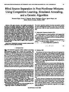
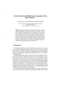
We created artificially four source signals, sparse of level 2, i.e. each column of the source matrix contains at least 2 zeros (shown in Figure 1). They are mixed with a square singular matrix A such that any 3 columns of it are linearly independent: −0.4326 −1.1465 0.3273 −1.2517 −1.6656 1.1909 0.1746 −0.3000 . A= 0.1253 1.1892 −0.1867 1.1278 0.2877 −0.0376 0.7258 0.9758 Since the mixing matrix is singular, the data lie on a hyperplane in R4 , i.e. in −1 a 3-dimensional subspace. We apply PCA: X1 = VX, where V = L3 2 UT3 , U3 is the matrix of those eigenvectors of XXT , which correspond to non-negative eigenvalues, XXT = ULUT and L3 is a diagonal matrix with the nonzero elements from L. So we obtain an overcomplete BSS problem X1 = A1 S with a (3 × 4) mixing matrix A1 = VA. After that we apply the matrix identification algorithm and source recovery algorithms from [4] (described in this paper in a more general case). The mixed sources are shown in Fig.2, the recovered sources by our algorithm are shown in Fig. 3. For a comparison we show the result of applying ICA and BSS algorithms: Fast ICA algorithm, JADE and SOBI (see Figures 4, 5 and 6 respectively). For a numerical evaluation of our algorithm, we compare the matrix B, estimation of A1 , produced by our algorithms (which has normalized columns - with norm 1) and the matrix A1 = VA after normalization of the columns:
6
0.0036 V = −0.0031 −0.0027 −0.3995 B = 0.9088 −0.1201 −0.3995 A2 = 0.9088 −0.1201
0.0049 −0.0011 0.0128 −0.0069 0.0019 0.0037 , 0.0021 0.0027 0.0002 0.3667 −0.9971 −0.0059 0.8309 −0.0099 −0.2779 , 0.4184 0.0760 0.9606 −0.0059 0.9971 0.3667 −0.2779 0.0099 0.8309 . 0.9606 −0.0760 0.4184
The normalized matrix A2 =normalized(VA) is different only by permutation of columns from B, which shows the good performance of our method.
5
Conclusion
We showed how to solve BSS problems of linear mixtures with singular matrices using sparsity of the source signals and presented sufficient conditions for their solvability. We presented two methods for that: 1) a general one (see matrix identification algorithm and source recovery algorithm) and 2) using reduction of the original problem to an overcomplete one, which we solve by sparse BSS methods. The presented computer simulation example shows the excellent separation by our algorithms, while the Fast ICA algorithm, JADE and SOBI algorithms fail.
References 1. A. Cichocki and S. Amari. Adaptive Blind Signal and Image Processing. John Wiley, Chichester, 2002. 2. P. Comon. Independent component analysis - a new concept? Signal Processing, 36: 287314, 1994. 3. J. Eriksson and V. Koivunen. Identifiability and separability of linear ica models revisited. In Proc. of ICA 2003, pages 2327, 2003. 4. P. Georgiev, F.J. Theis, and A. Cichocki. Blind source separation and sparse component analysis of overcomplete mixtures. In Proc. of ICASSP 2004, Montreal, Canada, 2004. 5. A. Hyv¨ arinen, J. Karhunen and E. Oja, Independent Component Analysis, John Wiley & Sons, 2001. 6. T.-W. Lee, M.S. Lewicki, M. Girolami, T.J. Sejnowski, “Blind sourse separation of more sources than mixtures using overcomplete representaitons”, IEEE Signal Process. Lett., Vol. 6, no. 4, pp. 87–90, 1999. 7. F.J. Theis, E.W. Lang, and C.G. Puntonet, A geometric algorithm for overcomplete linear ICA. Neurocomputing, in print, 2003. 8. K. Waheed, F. Salem, “Algebraic Overcomplete Independent Component Analysis”, in Proc. Int. Conf. ICA2003, Nara, Japan, pp. 1077–1082. 9. M. Zibulevsky, and B. A. Pearlmutter, “Blind source separation by sparse decomposition in a signal dictionary”, Neural Comput., Vol. 13, no. 4, pp. 863–882, 2001.
7 10 5 0 −5
0
500
1000
1500
2000
2500
3000
3500
4000
4500
5000
0
500
1000
1500
2000
2500
3000
3500
4000
4500
5000
0
500
1000
1500
2000
2500
3000
3500
4000
4500
5000
0
500
1000
1500
2000
2500
3000
3500
4000
4500
5000
5 0 −5 −10 5
0
−5 4 2 0 −2
Fig. 1. Original source signals. 10
0
−10
0
500
1000
1500
2000
2500
3000
3500
4000
4500
5000
0
500
1000
1500
2000
2500
3000
3500
4000
4500
5000
0
500
1000
1500
2000
2500
3000
3500
4000
4500
5000
0
500
1000
1500
2000
2500
3000
3500
4000
4500
5000
10 0 −10 −20 10
0
−10 5
0
−5
Fig. 2. Mixed signals. 0.2
0
−0.2
0
500
1000
1500
2000
2500
3000
3500
4000
4500
5000
0
500
1000
1500
2000
2500
3000
3500
4000
4500
5000
0
500
1000
1500
2000
2500
3000
3500
4000
4500
5000
0
500
1000
1500
2000
2500
3000
3500
4000
4500
5000
0.05
0
−0.05 0.05
0
−0.05 0.1
0
−0.1
Fig. 3. Estimated sources by our algorithms.
8 Estimated sources (independent components) 15 10
y1.
5 0 −5 0.2 0.1
y2.
0 −0.1 −0.2 4 2
y3.
0 −2 −4 4 2
y4.
0 −2 −4 0
500
1000
1500
2000
2500
3000
3500
4000
4500
5000
4000
4500
5000
4000
4500
5000
Fig. 4. Estimated sources by the Fast ICA algorithm. Estimated sources (independent components) 5
y1.
0
−5 5 0
y2.
−5 −10 −15 4 2
y3.
0 −2 −4 1 0.5
y4.
0 −0.5 −1 0
500
1000
1500
2000
2500
3000
3500
Fig. 5. Results by applying of JADE. Estimated sources (independent components) 4 2
y1.
0 −2 −4 5 0
y2. −5 −10 1 0.5
y3.
0 −0.5 −1 4 2
y4.
0 −2 −4 0
500
1000
1500
2000
2500
3000
3500
Fig. 6. Results by applying of SOBI.