Blind Source Separation with Compressively Sensed Linear Mixtures

Blind Source Separation with Compressively Sensed Linear Mixtures 1 Martin Kleinsteuber and Hao Shen October 13, 2011

arXiv:1110.2593v1 [cs.IT] 12 Oct 2011

Abstract This work studies the problem of simultaneously separating and reconstructing signals from compressively sensed linear mixtures. We assume that all source signals share a common sparse representation basis. The approach combines classical Compressive Sensing (CS) theory with a linear mixing model. It allows the mixtures to be sampled independently of each other. If samples are acquired in the time domain, this means that the sensors need not be synchronized. Since Blind Source Separation (BSS) from a linear mixture is only possible up to permutation and scaling, factoring out these ambiguities leads to a minimization problem on the so-called oblique manifold. We develop a geometric conjugate subgradient method that scales to large systems for solving the problem. Numerical results demonstrate the promising performance of the proposed algorithm compared to several state of the art methods. Index Terms

Compressed sensing, blind source separation, oblique manifold, conjugate subgradient method.

1

Introduction

Recovering signals from only the mixed observations without knowing the priori information of both the source signals and the mixing process is often referred to as Blind Source Separation (BSS), cf. [2]. Different BSS methods are used in various challenging data analysis applications, such as functional Magnetic Resonance Imaging (fMRI) analysis and microarray analysis. In order to achieve reasonable performance, prominent methods, e.g. Independent Component Analysis (ICA), usually require a large number of observations [3]. Unfortunately, the availability of a large amount of data samples can not be guaranteed in many real applications, due to either cost or time issues. The theory of compressed sensing (CS), cf. [4], shows that, when a signal is sparse (or compressible) with respect to some basis, only a small number of samples suffice for exact (or approximate) recovery. It is interesting to know that the concept of sparsity has also been used as a separation criterion in the context 1 M. Kleinsteuber and H. Shen are with the Department of Electrical Engineering and Information Technology, Technische Universit¨ at M¨ unchen, M¨ unchen, Germany. e-mail: (see http://www.gol.ei.tum.de). Authors are listed in alphabetical order due to equal contribution. Parts of this work have been presented at the Workshop Signal Processing with Adaptive Sparse Structured Representations (SPARS’11), Edinburgh, June 2011 [1]. This work has partially been supported by the Cluster of Excellence CoTeSys - Cognition for Technical Systems, funded by the Deutsche Forschungsgemeinschaft (DFG).

1

of BSS. In [5], for example, a family of efficient algorithms in the probabilistic framework are proposed. In [6], the authors investigate sparse representation of signals in an overcomplete basis in conjunction with BSS and motivate the usage of `1 -norm for a sparsity measure. The approach presented in this work can be regarded as a generalization of Morphological Component Analysis (MCA), cf. [7] and [8]. Roughly speaking, while MCA takes advantage of the sparse representations of the signals only for separation tasks, we additionally employ the sparsity assumption for reconstruction. The resulting cost function is thus very much related to the ones that typically arise in MCA. Nevertheless, the current scenario with compressively sensed samples has not been studied and thus differs from the existing MCA models. Although it has the potential of tackling the underdetermined BSS case, our numerical validation only considers the determined case, where the number of sources equals the number of mixtures. By considering the classical result that the source signals can only be extracted with scaling ambiguity, we regularize our problem by restricting each column of the mixing matrix to have unit norm. In other words, the resulting optimization problem is defined on the so-called oblique manifold. Furthermore, as many potential applications of the present work lie in the area of image or audio signal processing, any promising algorithms have to be capable of scaling to large systems. It is well known that conjugate gradient-type methods provide a nice trade-off between large scale problems and good convergence behavior. In this work, we propose an approach that lifts the conjugate subgradient method proposed by Wolfe in [9] to the manifold case. The paper is outlined as follows. Section 2 introduces some basic concepts and provides a description of the compressively sensed BSS problem. In Section 3, we develop a geometric subgradient algorithm. Finally, numerical results and conclusions are given in Section 4 and Section 5 respectively.

2 2.1

Problem Description Notation and Setting

For the sake of convenience of presentation, we follow the notation in the compressive sensing literature and represent the signals as column vectors. The instantaneous linear BSS model is given by Y = SA,

(1)

where S = [s1 , . . . , sm ] ∈ Rn×m denotes the data matrix of m sources with n samples (m  n), A = [a1 , . . . , ak ] ∈ Rm×k is the mixing matrix of full rank, and Y = [y1 , . . . , yk ] ∈ Rn×k represents the k linear mixtures of S. The task of standard BSS is to estimate the sources S, given only the mixtures Y . We assume that for all sources si ∈ Rn , there exists an (overcomplete) basis D ∈ Rn×d , n ≤ d, of Rn , referred to as representation basis, such that si = Dxi , with sparse xi ∈ Rd . More compactly, this reads as S = DX, where X = [x1 , . . . , xm ] ∈ Rd×m . 2

(2)

2.2

Compressively sensed BSS model

Now let us take one step further to compressively sample each mixture yi ∈ Rn individually. To this end, we denote the sampling matrix for the mixture yi by Φi ∈ Rpi ×n for i = 1, . . . , k. Then, a compressively sensed observation ybi ∈ Rpi of the i-th mixture is given by ybi = Φi yi = Φi DXai .

(3)

We refer to (3) as the Compressively Sensed BSS (CS-BSS) model. To summarize, the task considered in this work is formulated as: Given the compressively sensed observations ybi ∈ Rpi , for i = 1, . . . , k, together with their corresponding sampling matrices Φi ∈ Rpi ×n , estimate the mixing matrix A ∈ Rm×k and the sparse representations X ∈ Rn×m . There are various measures of sparsity available in the literature, cf. [10]. In this work, we confine ourselves to the `1 -norm as a measure of sparsity, because (i) it is suitable for numerical algorithms, in particular for large scale problems; (ii) it is an appropriate prior for many real signals, cf. [5]. This leads to the following optimization problem argmin kXk1 , s.t. ybi = Φi DXai , i = 1, . . . , k.

(4)

X,A

In real applications, it is unavoidable that the observations ybi are contaminated by noise. Hence let i denote the error radius for the observation i. The optimization problem (4) turns into argmin kXk1 , s.t. kb yi − Φi DXai k2 ≤ i , i = 1, . . . , k.

(5)

X,A

Following a standard approach, we formulate (5) in an unconstrained Lagrangian form, namely k X argmin kXk1 + λi kb yi − Φi DXai k22 , (6) X,A

i=1

where the scalars λi ∈ R+ weigh the reconstruction error of each mixture individually according to λi ∼ 1/2i , and balance these errors against the sparsity term kXk1 . It is well known that, in compressive sensing, inappropriate regularization parameters might lead to not only slow convergence but also local optima. To cope with this issue, we follow the adaptive updating strategy proposed in [11, 12]. A rigorous analysis of the updating strategy in our CS-BSS setting is beyond the scope of this work.

2.3

Regularized CS-BSS problem

Obviously, problem (6) is ill-posed. Indeed, an optimization procedure would let the norm of A explode to drive kXk1 to zero. In order to regularize the problem, we therefore restrict to the case where kai k2 = 1 for all i = 1, . . . , k. Thus, together with the full rank condition, we restrict the mixing matrix A onto the oblique manifold [13]  OB(m, k) := A ∈ Rm×k rk(A) = k, ddiag(A>A) = Ik , (7) 3

where Ik is the (k × k) identity matrix, and ddiag(Z) forms a diagonal matrix, whose diagonal entries are those of Z. Note, that this is a common approach in many BSS scenarios, since it is well known [14] that the mixing matrix A is identifiable only up to a column-wise scaling and permutation. The regularized problem that we will consider is hence given by argmin kXk1 + d×m

X∈R A∈OB(m,k)

k X

2

λi kb yi − Φi DXai k2 .

(8)

i=1

The optimization problem is thus defined on the product manifold Rd×m × OB(m, k).

3 3.1

A Conjugate Subgradient type method for the CS-BSS problem Conjugate Subgradient on Riemannian manifolds

In order to tackle the non-smooth problem (8), we propose a conjugate subgradient type approach on manifolds by generalizing the method proposed in [9]. A generalization of subgradient methods to the Riemannian manifold case has been studied in [15]. We refer to [16] for an introduction to nonsmooth analysis on manifolds, where the required concepts are introduced. Generally, for minimizing a nonsmooth function f : M → R where M is a Riemannian manifold and a subgradient of f exists for all x ∈ M , we propose the following scheme, further referred to as Riemannian Conjugate Subgradient (CSG) method. Let Tx M be the tangent space at x, let ∂f (x) ⊂ Tx M denote the Riemannian subdifferential of f at x, i.e. the set of all Riemannian subgradients at x, and let k · kR denote the norm on Tx M which is induced by the Riemannian metric h·, ·iR . Moreover, let G(x) := argmin kξkR (9) ξ∈∂f (x)

denote the subgradient with smallest Riemannian norm. Let x0 ∈ M be an initial point for the algorithm. Denote Gi := G(xi ), and the descent direction at the i-th iteration by Hi ∈ Txi M . By initializing H0 := −G0 , the algorithm now iteratively updates xi+1 = expxi (αi Hi ) , (10) where exp denotes the Riemannian exponential and the scalar αi is the line search parameter at the i-th iteration. Various line-search techniques for computing αi exist from which we choose backtracking line-search [17], cf. also [18] for the Riemmanian case, as it is conceptually simple and computationally cheap. There are also several formulas available that update the descent direction, e.g. Hestenes-Stiefel, PolakRibi`ere, and Fletcher-Reeves, which can all be generalized straightforwardly to the manifold setting. Here, we restrict to a manifold adaption of HestenesStiefel. Let ξ ∈ Txi M and denote by τi (ξ) ∈ Txi+1 M the parallel transport of 4

ξ along the geodesic γ(t) = expxi (tHi ) into the tangent space Txi+1 M . The direction update is then given by Hi+1 := −Gi+1 +

hGi+1 , Gi+1 − τi (Gi )iR τi (Hi ). hτi (Hi ), Gi+1 − τi (Gi )iR

(11)

Equations (10) and (11) are iterated until a stopping criterion is met. Usually, conjugate gradient methods use a reset after N = dimM iterations, i.e. Hi := −Gi if i mod N = 0. We propose to reset the direction when no significant update on the search directions is observed.

3.2

The Riemannian subgradient for CS-BSS

The manifold M = Rd×m × OB(m, k) is endowed with the Riemannian metric inherited from the surrounding Euclidean space, that is h(X1 , A1 ), (X2 , A2 )iR := tr(X1 X2> ) + tr(A1 A> 2 ).

(12)

Let λi > 0 for i = 1, . . . , k and let f : Rd×m ×OB(m, k) → R, f (X, A) = kXk1 +

k X

λi kb yi − Φi DXai k22 .

(13)

i=1

The Riemannian subdifferential of f at (X, A) with respect to the Riemmanian metric (12) is given by ∂f (X, A) = {(∂1 f (X, A), ∂2 f (X, A))},

(14)

where k X

λi (Φi D)>(Φi DXai −b yi ) a> i

(15)

  ∂2 f (X,A) = λi Π(ai )(Φi DX)>(Φi DXai −b yi ) i=1,...,k .

(16)

∂1 f (X, A) = ∂kXk1 +

i=1

and Here, ∂kXk1 = {H ∈ Rd×m | Hij = sign(Xij ) if Xij 6= 0, Hij ∈ [−1, 1] else}, and Π(ai ) := Im − ai a> i is an orthogonal projection operator. Note, that ∂2 f (X, A) is in fact a Riemannian gradient on the oblique manifold. Hence we may write ∂2 f (X, A) = ∇2 f (X, A). For the purpose of finding the subgradient with smallest Riemannian norm, each entry of ∂1 f (X, A) can be minimized independently. Let us denote the second summand at the right-hand side of (15) by k X B := λ i D > Φ> bi ) a> (17) i (Φi DXai − y i i=1

and define C ∈ Rd×m as the matrix with (i, j)-entries ( sign(Xij ) if Xij 6= 0 Cij := −sign(Bij ) min{|Bij |, 1} otherwise.

(18)

Then the subgradient G(X, A) ⊂ ∂f (X, A) having smallest Riemmanian norm is given explicitly by G(A, X) = (C + B, ∇2 f (X, A)) . 5

(19)

3.3

A Conjugate Subgradient Algorithm

The development of a Riemannian Conjugate Subgradient method requires the concept of parallel transport along a geodesic. Since we consider the oblique manifold as a Riemannian submanifold of a product of unit spheres, the formulas for the parallel transport as well as the exponential mapping read accordingly. Let ξ> ψ (20) τx,ξ (ψ) := ψ − kξk 2 (xkξk sin tkξk + ξ(1 − cos tkξk)) . be the parallel transport of a tangent vector ψ ∈ Tx S m−1 along the great circle γx,ξ (t) in the direction ξ ∈ Tx S m−1 on the unit sphere S m−1 , where γx,ξ : R → S m−1 , ( x, γx,ξ (t) := tkξk , x cos tkξk+ ξ sinkξk

kξk = 0; otherwise.

(21)

Then the parallel transport of (H, Ψ) ∈ T(X,A) Rd×m × OB(m, k) with respect to the Levi-Civita connection along the geodesic γ(X,A) in the direction (Z, Ξ) ∈ T(X,A) Rd×m × OB(m, k), i.e. γ(X,A) : R → Rd×m × OB(m, k), γ(X,A) (t) := (X + tZ, [γai ,ξi (t)]i=1,...,k )

(22)

is given by   τ(X,A),(Z,Ξ) (H, Ψ) := H, [τai ,ξi (ψi )]i=1,...,k .

(23)

A conjugate subgradient algorithm for the problem as defined in (8) is summarized as follows. Algorithm 1 A conjugate subgradient CS-BSS algorithm Step 1: Initialize X (0) ∈ Rd×m and A(0) ∈ OB(m, k). Set i = 0. Step 2: Set i = i + 1, let X (i) = X (i−1) and A(i) = A(i−1) , and compute G(1) = H (1) = −G(A(i) , X (i) ). Step 3: For j = 1, . . . , d · m + m(m − 1) − 1:
(i) Update X (i) , A(i) ← γ(X (i) ,A(i) ),H (i) (λ∗ ), where λ∗ = argmin γ(X (i) ,A(i) ),H (i) (λ); λ∈R

(ii) Compute G(j+1) = −G(A(i) , X (i) ); (iii) Update H (j+1) ← G(j+1) + µ τ(X (i) ,A(i) ),H (j) (H (j) ), where µ is chosen according to (11);

(iv) If H (j+1) − H (j) is small enough, go to Step 2.



Step 4: If A(i+1) − A(i) + X (i+1) − X (i) is small enough, stop. Otherwise, go to Step 2.

6

4

Numerical Results

0.7

50

0.6

40

0.5

SNR (dB)

Amari error

30 0.4

0.3

20

10 0.2 0

0.1

0

−10 CSG

Smoothing CG

Alt−CG−CSG

Alt−IHT

Alt−IST

CSG

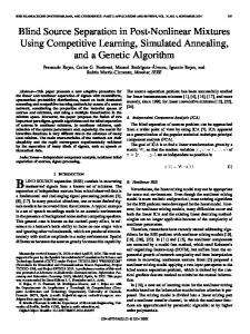
(a) Comparison in terms of Amari error

Smoothing CG

Alt−CG−CSG

Alt−IHT

Alt−IST

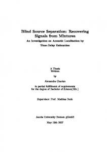
(b) Comparison in terms of SNR

Figure 1: Experimental results. In our experiment, we investigate the performance of the proposed CSG algorithm compared with several state of the art algorithms. By noticing the similarity between our present work with the generalized MCA method in [8], we adapt the alternating soft-thresholding based method and the hard thresholding [19] (where `0 is used as a sparsity measure) to our CS-BSS setting. We refer to them as Alt-IST and Alt-IHT, respectively. Similarly, we adapt the CSG algorithm in the alternating manner (referred to as Alt-CG-CSG). Finally, one alternative common approach to deal with the nondifferentiability of the cost function is to employ a smooth approximation. We then refer to the standard CG algorithm with certain smooth approximation as smoothing CG. In the experiment, we generate three sources signals with n = 1000 samples. The number of nonzero entries is equal to 100, which are generated according to a Laplacian distribution. We randomly pick 300 samples as the compressively sensed mixtures. The performance is measured in terms of both separation quality, measured by the Amari Error [20], and reconstruction quality in terms of Signal to Noise Ratio (SNR). Figure I illustrates the box plot of the results from 50 experiments of all methods. Among all five methods, the Alt-CG-CSG performs the worst on average in terms of both separation and reconstruction qualities, while the proposed CSG algorithm provides consistent and satisfactory results. Finally, the small variances of all CG/CSG type algorithms in terms of reconstruction also suggest their reliable performance compared with the thresholding based approaches.

5

Conclusion

In this work, the authors propose a method for separating linearly mixed sparse signals from compressively sensed mixtures. The proposed approach allows each mixture to be sensed individually. If sampling takes place in the time domain, this means that the sensors do not have to be synchronized. The arising optimization problem is tackled with a conjugate subgradient type method, which is based on a new concept for optimizing non-differentiable functions under smooth constraints. 7

References [1] M. Kleinsteuber and H. Shen, “Blind source separation of compressively sensed signals,” in Proceedings of the 4th Workshop on Signal Processing with Adaptive Sparse Structured Representations, 2011, p. 80. [2] S. Haykin, Unsupervised Adaptive Filtering. Wiley-Interscience, 2000, vol. 1: Blind Source Separation. [3] S. Bermejo, “Finite sample effects in higher order statistics contrast functions for sequential blind source separation,” IEEE Signal Processing Letters, vol. 12, no. 6, pp. 481–484, 2005. [4] D. L. Donoho, “Compressed sensing,” IEEE Transactions on Information Theory, vol. 52, pp. 1289–1306, 2006. [5] M. Zibulevsky and B. A. Pearlmutter, “Blind source separation by sparse decomposition in a signal dictionary,” Neural Computation, vol. 13, no. 4, pp. 863–882, 2001. [6] Y. Li, A. Cichocki, and S.-i. Amari, “Analysis of sparse representation and blind source separation,” Neural Computation, vol. 16, pp. 1193–1234, 2004. [7] M. Elad, J. Starck, P. Querre, and D. l. Donoho, “Simultaneous cartoon and texture image inpainting using morphological component analysis (MCA),” Applied and Computational Harmonic Analysis, vol. 19, no. 3, pp. 340–358, 2005. [8] J. Bobin, J.-L. Starck, J. Fadili, and Y. Moudden, “Sparsity and morphological diversity in blind source separation,” IEEE Transactions on Image Processing, vol. 16, no. 11, pp. 2662 –2674, 2007. [9] P. Wolfe, “A method of conjugate subgradients for minimizing nondifferentiable functions,” in Nondifferentiable Optimization, ser. Mathematical Programming Studies, 1975, vol. 3, pp. 145–173. [10] N. Hurley and S. Rickard, “Comparing measures of sparsity,” IEEE Transactions on Information Theory, vol. 55, no. 10, pp. 4723 –4741, 2009. [11] J. Bobin, J. Starck, J. M. Fadili, Y. Moudden, and D. L. Donoho, “Morphological component analysis: An adaptive thresholding strategy,” IEEE Transactions on Image Processing, vol. 16, no. 11, pp. 2675–2681, 2007. [12] S. J. Wright, R. D. Nowak, and M. A. T. Figueiredo, “Sparse reconstruction by separable approximation,” IEEE Transactions on Signal Processing, vol. 57, pp. 2479–2493, 2009. [13] H. Shen and M. Kleinsteuber, “Complex blind source separation via simultaneous strong uncorrelating transform,” in Lecture Notes in Computer Science, Proceedings of the 9th International Conference on Latent Variable Analysis and Signal Separation” (LVA/ICA 2010), vol. 6365. Berlin/Heidelberg: Springer-Verlag, 2010, pp. 287–294. 8

[14] P. Comon, “Independent component analysis, a new concept?” Signal Processing, vol. 36, no. 3, pp. 287–314, 1994. [15] O. P. Ferreira and P. R. Oliveira, “Subgradient algorithm on Riemannian manifolds,” Journal of Optimization Theory and Applications, vol. 97, pp. 93–104, 1998. [16] Y. S. Ledyaev and Q. J. Zhu, “Nonsmooth analysis on smooth manifolds,” Transactions of the American Mathematical Society, vol. 359, no. 8, pp. 3687–3732, 2007. [17] J. Nocedal and S. J. Wright, Numerical Optimization, 2nd Ed. New York: Springer, 2006. [18] P.-A. Absil, R. Mahony, and R. Sepulchre, Optimization Algorithms on Matrix Manifolds. Princeton, NJ: Princeton University Press, 2008. [19] T. Blumensath and M. E. Davies, “Iterative hard thresholding for compressed sensing,” Applied and Computational Harmonic Analysis, vol. 27, no. 3, pp. 265–274, 2009. [20] S. Amari, A. Cichocki, and H. H. Yang, “A new learning algorithm for blind signal separation,” Advances in Neural Information Processing Systems, vol. 8, pp. 757–763, 1996.

9