Ahtract- Nerve cuff Electrodes record an aggregate signal from a nerve comprised of several fascicles. Recovering individual fascicular signals could be ...
-
Proceedings of the 25* Annual International Conference of the IEEE EMBS Cancun, Mexico September 17-21,2003
Blind Source Separation of Nerve Cuff Recordings W. Tesfayesus', P. Yoo2, D. M. Durand3 ''2,3Departmentof Biomedical Engineering, Case Westem Reserve University, Cleveland, OH, USA
Ahtract- Nerve cuff Electrodes record an aggregate signal from a nerve comprised of several fascicles. Recovering individual fascicular signals could be important for the control of prosthetic devices. Blind Source Separation methods have been designed for recovering individual source signals from multi-channel recordings of a mixture of multiple sources. Here, we present a simulation study of the feasibility of applying Blind Source Separation (BSS) to recover fascicular signals from multiple contact nerve cuff electrodes. Spontaneous neuroelectric activities and their recordings are simulated. Hyvarinen's FastICA algorithm, a popular method for BSS, combined with a correlation analysis is used for separation. The ability of the method to separate the fascicular signals was estimated by measuring the correlation between the input and output signals. In 25 random trials with different signals the mean value of the correlation coefficient was 0.86 (k 0.15 S.D.). Although all signals were recovered every time, the algorithm was not able to determine the origin of the signals. The BSS procedure permutes separated signals randomly.
fascicular signals assuming fascicular signals are independent, and neural recordings a linear mixture of the fascicular signals. As far as we know, this is the first time BSS is being used for the separation of simulated recordings of spontaneous peripheral neuroelectric activity. 11. METHODOLOGY 1) Simulation: A spontaneous fascicular signal is simulated as a stochastic process. A triphasic compound action potential, AF'(t), with a lms duration and representing the signal from a small subpopulation of nerve fibers was generated using a motoneuron axon model in Neuron [6]. The fascicular signal s(t) is then the sum of randomly delayed AP(t) with a uniformly distributed random delay on a 100 ms interval [12]. N
S(t,tOl,
Keywords-Nerve Cuff Recordings, Independent Component Analysis, Blind Source Separation, Control Signals
I. INTRODUCTION Electrical stimulation of nerves can be used in motor prosthesis to partially restore movements to individuals with neurological impairments due to spinal cord injury or stroke [ 5 ] . Spontaneous fascicular electrical activities during relay of either sensory or motor information could be used as control signals for such prosthetic devices. For this purpose, different designs of nerve cuff electrodes have emerged, including the Flat Interface Nerve Electrode (FINE), which improve fascicular selectivity of neural recordings[ 141 [ 191. Nerve cuff electrodes record an aggregate signal from the entire nerve. These whole nerve recordings are signals that can be modeled as linear combinations of the electrical activity of active fibers within various fascicles [l 11. In order to recover neural signals from individual fascicles, we have analyzed neural recordings with a Blind Source Separation (BSS) method. BSS has been successfully applied in many biomedical applications including the removal of ECG artifacts from EEG recordings [20]. In Blind Source Separation analysis, an array of linearly mixed multiple independent sources is separated into an array of the original independent sources. In this paper we test the hypothesis that it is possible to separate the multi-channel nerve cuff recordings into the
0-7803-7789-3/03/$17.0002003 IEEE
'.'?t,N)
(1)
=xAP(t-tO,) 1=1
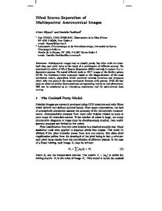
From the central limit theorem, s(t) should have a Gaussian distribution. A Kolmogorov-Smirnov test is applied to verify the distribution. When the fascicle is not active, background noise is simulated by adding a uniformly distributed random signal. Figure 1 shows a simulated fascicular signal and a typical raw electroneurogram which is shown to have a Gaussian distribution in [12]. 1N I
I
I
I
0
I
50
100
Time (111s)
Isn
0 '
1
2
3
4
Time (seconds)
Fig 1. (a) Simulated fascicular signal. The region during which the fascicle is active has Gaussian distribution. (b) Experimental recorded nerve signal [I61
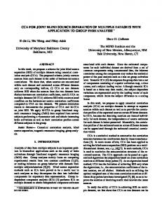
A finite element model was implemented to simulate the linear mixing of spontaneous fascicular signals. A nerve with four fascicles of differing radii (figure 2.a) and submerged in Saline (figure 2.b) was modeled. The conductivities were 0.0826 S/m radial and ,5714 S/m longitudinal for endoneurium, 0.0826 S/m for epineurium, 0.0021 S/m for perineurium, 2 S/m for saline, and l o 7 S/m for silicone (used to make the cuff electrodes). A fascicular
2507
signal s(t) generated as indicated above is used to simulate fascicular activity. The simulation generated a potential distribution all over the surface of the cuff electrode fkom which tripolar recordings at six contact points were extracted.
Fig. 2. Geometry of simulated nerve submerged in saline. (a) The nerve
comprised of four fascicles with the FINE electrode wrapped around it. (b) The nerve submerged in Saline bath (D = 6mm and L = 60mm).
Cuff electrode recordings, with single or several active fascicles, were simulated. Different fascicles may be active simultaneously or delayed from each other. Cuff electrode recordings with several active fascicles were obtained by calculating the potential distributions over the electrode for each fascicle active and adding them. Electrode recordings representing potentials at a given number of contact points on the electrode are then calculated for tripolar mode of recording 2) The ICA Algorithm: When N independent signals are linearly mixed and recorded using an array of M electrodes, BSS can be used to individually separate and identify the original independent sources fiom the recordings. All N independent signals can be separated only if M L N. The array of recorded signals x(t) can be written in terms of the original source signals s(t), the mixing matrix A , and recorded noise n(t) as x(' = As(t) + n(t) (2) The approximated independent sources a(t) would then be a(t) = Wx(t) (3) where W is a matrix that either maximizes the nongaussianity of the elements of a(t) [8] or a first stage linear transformation in a two-stage mapping implemented by a single layer feed-forward neural network. The second stage of the mapping is Y(t) = g(a(t)) (4) where g is a bounded nonlinearity. The mapping f x y is one that maximizes the information transmitted [3]. In cases where the number of recording channels M is greater than number of source signals N preprocessing methods such as Principal Component Analysis (PCA) can be used to estimate the dimension of the source signals. In Blind Source Separation, PCA also reduces the number of
-
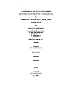
unknown parameters of W significantly increasing the speed of the algorithm. The de-mixing matrix W relates to the mixing matrix A as w = PDA-I (5) The above relation indicates that the separated signals are nearly equal to the source signals s(t) within a permutation and scaling. In addition, the order of the elements of a(t) changes every time BSS is done. If the separated signals are to be used as control signals, it is important that each separated signal be associated deterministically to a recording channel and hence to a fascicle assuming a fascicle is spatially stationary. In our case, the vector x(t) represents the channel recordings, s(t) the fascicular signals, and a(t) the separated signals. Since there were four fascicles and six recording channels, s(t) and x(t) had four and six elements respectively. The performance of BSS, i.e. how close the elements of a(t) are to the elements of so) can be quantified by calculating the correlation coefficient between each element of a(t) and s(t). When a separated signal, say a!, is an estimation of a given element of s(t), say s2,the correlation coefficient between a1 and s2 will be higher than that between a1 and the rest of the elements of s(t). The higher the correlation coefficient between al and s2 the better the performance of BSS. Before calculating the correlation coefficients, the elements of s(t), x(t), and a(t) are rectified and a moving average (window of 10 ms) signal is obtained. 111. Results Four fascicular signals with various delays and duration, of the active region, were generated (fig.1). The fascicular signals were rectified and h e integrated signals are shown in figure 3.a. The fascicular signals were then entered into the model simulating a nerve cuff recording. The recorded signals, at the six contact points, were also rectified and the integrated signals, shown in figure 3.b, obtained. The recorded signals were separated using FastICA into estimations of the fascicular signals. On a 2.8 GHz P4 computer, separation of a 200ms signal sampled at a 1000 points was achieved in under 150 ms. The separated signals were rectified and integrated and are shown in figure 3.c. ICA separated the recorded signals into a vector a(t) of six elements. The active regions present in the fascicular signals, figure 3.a, can be easily recognized in the separated signals, figure 3.c. Figure 3.c also shows that all four of the fascicular signals have been separated. However, the PCA did not eliminate the independent signals and two additional signals are separated by the algorithm.
2508
To evaluate the separation procedure three aspects have been considered: 1) the accuracy of separation. 2 ) independence of separated signals. 3) elimination of permutation ambiguity.
TABLE I CORRELATION COEFFICIENTS BETWEEN ORIGINAL AND SEPARATED
.CI
Fascicular Signals s ( t ) SI s2 s3 s4 10.04
1 0.52
I
,
I-0.081 0.63 0.40 0.47 0.42 1-0.22 I To test the independence of the recovered signals, the correlation coefficient between the separated signals was calculated. We note here that the correlation coefficient between the separated signals and the fascicular signals cannot be calculated in practice since the fascicular signals are unknown. When the correlation of two signals is higher than a threshold value (0.7 based on the distribution of correlation coefficient values) one of the signals is eliminated. For example, u2 and u4 in figure 3.c were eliminated since they both had high correlation with a3 and a5respectively. Using this procedure, the four original signals were recovered every time in 25 trials. However, it was not possible to relate the separated signals to the sources since the procedure permutes the signals randomly. Therefore the permutation ambiguity remains to be solved. Fig 3. Rectified and averaged (moving) fascicular (a), recordings (b), and separated signals (c). The active regions of the fascicles can clearly be seen in the fascicular and separated signals.
To quantify the accuracy of BSS the correlation coefficients between the separated signals, up), and the fascicular signals, sp), were calculated. The correlation coefficient values for the signals in figure 3 are shown in Table I. The correlation coefficient is highest when an element of up) is an estimation of an element of s(t) (shaded cells in table I). The mean value of the highest correlation coefficient between elements of a(t) and s(f) is 0.85. To test the robustness of BSS, twenty five trials were conducted. In each trial, four fascicular signals, with random delay and duration, were generated, mixed in the finite element model and separated using ICA. The mean values and the standard deviations of the highest correlation coefficients were 0.86 and 0.15 respectively.
IV. DISCUSSION Separation of a six channel recording, xfi), resulted in six signals, u(t), while there were only four source signals, s(t). This means that pre-ICA processing method, Principal Component Analysis, did not reduce the dimensions of the mixed signals. This could be explained by the fact that the covariance matrix of the mixed signals is of full rank due to the small spacing between the contact points. Therefore post ICA processing has to be done to find the dimensions of the source signals. Here, we show that calculating the correlation coefficient between the separated signals can eliminate similar signals. This simulation study shows that it might be possible to use ICA for the separation of multi-channel nerve cuff recordings. With ICA, four independent source signals can be hlly separated in the model described with four signals
2509
and six contact points. On-line implementation of ICA to obtain control signals is also possible since the FastICA algorithm [8] has the necessary speed. However, separated signals, elements of a(t), could not be related to recording channels, x,, due to ICA’s permutation ambiguity. To overcome this problem, we intend to investigate the use of complementing ICA with an inverse problem analysis.
V. Conclusion The blind separation method described here can eliminate fascicular signals fascicular signals with high correlation. PCA did not reduce the dimensions of recorded signals. A correlation analysis applied after the separation was used successfully instead. The permutation ambiguity of ICA prevents identification of a recovered signal with its source.
ACKNOWLEDGMENT The authors would like to thank Michael Moffitt. Financial support was provided by NIH grant NS 32855 and the Department of Education G A A ” fellowship program.
REFERENCES
S. Amari et al. “Blind Signal Separation and Extraction: Neural and InformationTheoretic Approaches” Chap 3. Unsupervised Adaptive Filtering. Vol 1 ; Simon Haykin, editor. 2000 B. Azzerboni et. al. “Spatio-temporal Analysis of Surface Electromyography Signals by Independent Component Timescale Analysis.” Proceedings of the Second EMBSBMES Joint Conference, Houston, TX, USA. October 23-26, 2002. Bell & Sejnowski “An information maximization approach to blind separation and blind deconvolution.” Neural Computation, 7(6), 1129-1159,1995 A. Belouchrani et. al. “A Blind Source Separation Technique Using Second Order Statistics.” IEEE Transactions on Signal Processing, 45(2): 434444, 1997 W.M. Grill & R. F. Kirsch, “Neuroprosthetic Applications of Electrical Stimulation. ” Asst. Technol, 12:6-20, 2000 M. L. Hines and N. T. Carnevale, “The NEURON simulation environment,” Neural Comput., vol. 9, pp. 1 1 79-1 209, 1997. A. Hyvarinent‘The FastICA MATLAB toolbox.” Helsinki Univ. ofTechnology. 1998 A. Hyvarinen, “Fast and robust fixed-point algorithms for independent component analysis. IEEE Transactions on Neural Networks, 10(3), 626-634, 1999 A. Hyvarinen “Fast ICA by a fixed-point algorithm that maximizes non-Gaussianity” Chap 2, Independent Component Analysis, Stephen Roberts, editor; 2001 [IO] D. Iyer et al. “Independent Component Analysis of Multichannel Auditory Evoked Potentials.” Proceedings of the ”
25 10
Second Joint EMBSBMES Conference. Houston, TX, USA. October 23-26,2002. [ I I ] S . Jezemik & W. M. Grill “Optimal Filtering of Whole Nerve Signals.” Journal of Neuroscience Methods, 106: 101 -1 IO, 2001
[I21 S. Jezemik & Thomas Sinkjaer “On statistical Properties of whole nerve cuff rec:ordings”ZEEE TBME, Vo1.46, No. 10, October 1999 [I31 K.G. Oweiss & D.J. Anderson. “Independent Component Analysis of Multichannel Neural Recordings and the Microscale.” Proceedings cif the Second EMBSBMES Conference. Houston, TX, USA. October 23-26,2002, [I41 J. Perez-Orive & DM Durand “Modeling Study of Peripheral Nerve Recording Selectivity” IEEE Trans Rehabil Eng, 8(3):320-9, Sep 2000 [ 151 J. Rozman et. al. “Selective Recording of Neuroelectric Activity From the Peripheral Nerve.” European Journal of Physiology, 44O[~~ppl]: R157-R159,2000 [16] M. Sahin “Chronic Recordings of Hypglossal Nerve in a Dog Model of Upper Airuay Obstruction” ?‘h.D. Thesis May 1998 CWRU [17] R. B. Stein. et. al. “Principles Underlying New Methods for Chronic Neural Recording.” Le Journal Canadien Des Sciences Neurologiques, 235-244, 1975. Available: http://www (URL) [I 81 M. Valencia et. al. “!;omatosensory Evoked Potentials Sources Revealed by ICA.” Proceedings of the Second Joint EBMSBMES Conference. Houston, TX, USA. October 23-26, 2002 [ 191 P. Yo0 et al. “Selectivi: Fascicular Recording of the Hypoglossal Nerve Using a Multi-Contact Nerve Cuff Electrode” Proceedings of EMBC, Cancun, Mexico, Sep 2003 [20] W. Zhou “Removal cf ECG Artifacts from EEG Using ICA.” Proceedings of the !Second Joint EMBSBMES Conference, Houston, TX, USA. October 23-26,2002,