blind source separation using time-frequency distributions ... - CiteSeerX

BLIND SOURCE SEPARATION USING TIME-FREQUENCY DISTRIBUTIONS: ALGORITHM AND ASYMPTOTIC PERFORMANCE. Adel Belouchrani and Moeness G. Amin Department of Electrical and Computer Engineering, Villanova University, Villanova PA 19085 USA

x(t) denotes the output of the sensors at time instant t which may be corrupted by an additive noise n(t). Hence,

ABSTRACT

This paper addresses the problem of the blind source separation which consists of recovering a set of signals of which only instantaneous linear mixtures are observed. A blind source separation approach exploiting the dierence in the time-frequency (t-f) signatures of the sources is considered. The approach is based on the diagonalization of a combined set of `spatial time-frequency distributions'. Asymptotic performance analysis of the proposed method is performed. Numerical simulations are provided to demonstrate the effectiveness of our approach and to validate the theoretical expression of the asymptotic performance.

the linear data model is given by:

x(t) = As(t) + n(t);

where the m  n matrix A is called the `mixing matrix'. The n source signals are collected in a n  1 vector denoted s(t)

which is referred to as the source signal vector. The sources are assumed to have dierent structures and localization properties in the time frequency domain. The mixing matrix A is full column rank but is otherwise unknown. In contrast with traditional parametric methods, no speci c structure of the mixture matrix is assumed. The problem of blind source separation has two inherent ambiguities. First, it is not possible to know the original labeling of the sources, hence any permutation of the estimated sources is also a satisfactory solution. The second ambiguity is that it is inherently impossible to uniquely identify the source signals. We take advantage of the second indeterminacy by treating the source signals as if they have unit power. This normalization still leaves undetermined the ordering and the phases of the columns of A. Hence, the blind source separation is a technique for the identi cation of the mixing matrix and/or the recovering of the source signals up to a xed permutation and some complex factors.

1. INTRODUCTION

Blind source separation consists of recovering a set of signals of which only instantaneous linear mixtures are observed. The rst solution to this problem was based on the cancellation of higher order moments assuming non-Gaussian and i.i.d. source signals [1]. Since then, other criteria based on minimizations of cost functions, such as the sum of square fourth order cumulants [2, 3], contrast functions [2] or likelihood function [4], have been used by several researchers. In the case of non i.i.d. source signals and even Gaussian sources, solutions based on second order statistics are possible [5, 6]. Matsuaka et al. have shown that the problem of the separation of nonstationary signals can be solved using second order decorrelation only [7]. They implicitly use the nonstationarity of the signal via a neural net approach. Herein, we propose to take advantage explicitly of the nonstationarity property of the signals to be separated. This is done by resorting to the powerful tool of time frequency signal representations. In this paper, we develop an approach based on a joint diagonalization of a combined set of spatial time-frequency distributions. This approach exploits the dierence between the t-f signatures of the sources. In contrast to existing methods, the proposed approach allows the separation of Gaussian sources with identical spectra shape but with different time-frequency localization properties. Moreover, the eects of spreading the noise power while localizing the source energy in the time-frequency domain amounts to increase the robustness of the proposed approach with respect to noise.

3. SPATIAL TIME-FREQUENCY DISTRIBUTIONS

The discrete-time form of the Cohen's class of timefrequency distributions (TFD), for signal x(t), is given by [8]

Dxx (t;f ) =

1 X l;m=?1

(m; l)x(t + m + l)x (t + m ? l)e?j4fl

(2) where t and f represent the time index and the frequency index, respectively. The kernel (m; l) characterizes the distribution and is a function of both the time and lag variables. The cross-TFD of two signals x1 (t) and x2 (t) is de ned by

2. PROBLEM FORMULATION

Consider m sensors receiving an instantaneous linear mixture of signals emitted from n sources. The m  1 vector

Dx1 x2 (t; f ) =

This work is supported by Rome Lab, NY, contract # F30602-96-C-0077.

To appear in Proc. ICASSP-97

(1)

1

1 X l;m=?1

(m; l)x1 (t+m+l)x2 (t+m?l)e?j4fl (3)

c IEEE 1997

favorable when considering simultaneous diagonalization of a combined set fDzz (ti ; fi )ji = 1;


; pg of p STFD matrices. This amounts to incorporating several time-frequency points in the source separation problem. It is noteworthy that two source signals with identical t-f signatures can not be separated even with the inclusion of all information in the t-f plane.

Expressions (2) and (3) are now used to de ne the following data spatial time-frequency distribution (STFD) matrix,

Dxx (t; f ) =

1 X

l;m=?1

(m; l)x(t + m + l)x (t + m ? l)e?j4fl

(4) where [Dxx (t; f )]ij = Dxi xj (t; f ); for i; j = 1;


; n. Under the linear data model of equation (1) and assuming noise-free environment, the STFD matrix takes the following simple structure:

Joint diagonalization: The joint diagonalization [6] can be explained by rst noting that the problem of the diagonalization of a single n  n normal matrix M is equivalent to the minimization of the criterion [11]

Dxx (t; f ) = ADss (t;f )AH

(5) where Dss (t; f ) is the signal TFD matrix whose entries are the auto- and cross-TFDs of the sources. We note that Dxx (t; f ) is of dimension m  m, whereas Dss(t; f ) is of n  n dimension. For narrowband array signal processing applications, matrix A holds the spatial information and maps the auto- and cross-TFDs of the sources into autoand cross-TFDs of the data. Since the o-diagonal elements of Dss(t; f ) are crossterms, then this matrix is diagonal for each time-frequency (t-f) point which corresponds to a true power concentration, i.e. signal auto-term. In the sequel, we consider the t-f points which satisfy this property. In practice, to simplify the selection of auto-terms, we apply a smoothing kernel (m; l) that signi cantly decreases the contribution of the cross-terms in the t-f plane. This kernel can be a member of the reduced interference distribution (RID) introduced in [9] or signal-dependent which matches the underlying signal characteristics [10].

C (M; V) def =?

X

i

jvi Mvi j2

(8)

over the set of unitary matrices V = [v1 ;


; vn ]. Hence, the joint diagonalization of a set fMk jk = 1::K g of K arbitrary n  n matrices is de ned as the minimization of the following JD criterion:

C (V) def =?

X

k

C (Mk ; V) = ?

X

ki

jvi Mk vi j2

(9)

under the same unitary constraint. An ecient joint approximate diagonalization algorithm exists in [6] and it is a generalization of the Jacobi technique [11] for the exact diagonalization of a single normal matrix.

Identi cation Procedure: Equations (5-9) constitute the blind source separation approach based on TFD which is summarized by the following steps ^ from the eigende Determine the whitening matrix W composition of an estimate of the covariance matrix of the data (see [6] for more details).  Determine the unitary matrix U^ by minimizing the joint approximate diagonalization criterion for a speci c set of whitened TFD matrices fDxx (ti ; fi )ji = 1;


; pg,  Obtain an estimate of the mixture matrix A^ as A^ = ^ #U ^ , where the superscript # denotes the pseudoW inverse, and an estimate of the source signals s^(t) as ^s(t) = U^ H Wx(t).

4. PROPOSED ALGORITHM Let W denotes a m  n matrix, such that (WA)(WA)H = UUH = I, i.e. WA is a mm unitary matrix (this matrix is

referred to as a whitening matrix, since it whitens the signal part of the observations). Pre- and post-multiplying the TFD-matrices Dxx (t; f ) by W, we then de ne the whitened TFD-matrices as: Dxx (t; f ) = WDxx (t; f )WH (6) From the de nition of W and Eq.(5), we may expressed Dxx (t; f ) as

Dxx (t;f ) = UDss (t;f )UH (7) Since the matrix U is unitary and Dss(t; f ) is diagonal, expression (7) shows that any whitened data STFD-matrix is diagonal in the basis of the columns of the matrix U (the eigenvalues of Dxx (t; f ) being the diagonal entries of Dss(t; f )). If, for the (ta; fa ) point, the diagonal elements of Dss(ta ; fa ) are all distinct, the missing unitary matrix U

5. ASYMPTOTIC PERFORMANCE

The performance is characterized in terms of signal rejection. After identi cation of the matrix A, the estimated source signals may be obtained as ^s(t) = A^ # x(t) = A^ # As(t) + A^ # n(t). The matrix P^ de ned by P^ = A^ # A should be close to some matrix P with only one zero phase term in each row and each column (phase and permutation indeterminacies). For convenience, we assume that P^ is close to a diagonal rather than to some other permutation matrix. The p-th estimated source signal is

may be `uniquely' (i.e. up to permutation and phase shifts) retrieved by computing the eigendecomposition of Dzz (ta; fa). However, when the t-f signatures of the dierent signals are not highly overlapping or frequently intersecting, which is likely to be the case, the selected (ta; fa) point often corresponds to a single signal auto-term, rendering matrix Dss(ta ; fa ) decient. That is, only one diagonal element of Dss(ta ; fa ) is dierent from zero. It follows that the determination of the matrix U from the eigendecomposition of a single whitened data STFD-matrix is no longer `unique' in the sense de ned above. The situation is more

^sp (t) =

n X q=1

P^pq sq (t) + (A# n(t))p

(10)

The power of the q-th source signal residual (interference) in the p-th estimated source signal is: Ipq = E jP^ pq j2 (since 2

 If the sources p and q have identical t-f signatures over the chosen t-f points (i.e. dp = dq ), the corresponding ISR Ipq ! 1.  As the correlation function rT pq of the sources p and q and the cross-terms Ds s (tk ; fk ) vanish, the corresponding ISR given by Ipq also vanishes, yielding a

the sources have unit power, this quantity is nothing but the interference to signal ratio (ISR) for the q and p-th source). As a global measure of performance, we use the overall rejection level de ned as the sum of all the interferences

Iperf def =

X

q6=p

E jP^ pq j2 =

X

q6=p

Ipq

p q

(11)

perfect separation.

 Ipq0 is independent of the mixing matrix. In the array

In the case of Gaussian noise and deterministic source signals, we have derived closed form expressions of the rejection index at the limit of large snapshots. Details of the calculation are presented in [12].

Ipq = Ipq0 + 2 Ipq1 + 4 Ipq2

processing context, it means that performance in terms of interference rejection are unaected by the array geometry. The performance depends only on the sample size and the t-f signatures of the sources.

6. PERFORMANCE EVALUATION Numerical experiments: we consider a uniform linear

(12)

where the coecients of the expansion are "

K X

0 = 1 2pq jrT pq j2 ? pq pqk rT pq Dsq sp (tk ;fk )+ Ipq 4 k=1 

rT qp Dsp sq (tk ;fk ) + "

K X

k;l=1

array of three sensors having half wavelength spacing and receiving signals from two sources in the presence of white Gaussian noise. The sources arrive from dierent directions 1 = 0 and 2 = 20 degrees. The source signals are generated by ltering a complex circular white Gaussian processes by an AR model of order one with coecient a1 = 0:85 exp(j 2f1 (t)) and a2 = 0:85 exp(j 2f2 (t)), where we have: ( 0:0625 for t = 1 : 400 0:1250 for t = 401 : 450 f1 (t) = 0:3750 for t = 451 : 850 ( 0:3750 for t = 1 : 400 0:1250 + f for t = 401 : 450 f2 (t) = 0:0625 for t = 451 : 850 The signal to noise ratio (SNR) is set at 5 dB. The kernel used for the computation of the TFDs is the Choi-Williams kernel [8] , which provides a good reduction of the crossterms. Eight TFD matrices are considered. The corresponding t-f points are those of the highest power in the t-f domain. The mean rejection level is evaluated over 500 Monte-Carlo runs. Table 1 shows the mean rejection level in dB versus the `spectral shift' f both for SOBI algorithm [6] and the new algorithm. Note that for f = 0, the two Gaussian source signals have identical spectra shape. In this case, while SOBI fails1 in separating the two sources, the proposed algorithm succeed.



#

pqk pql Dsp sq (tk ;fk )Dsq sp (tl ;fl )

K 1 = 1 2pq (rT pp Jqq + rT qq Jpp ) ? X pq pqk rT pq Jqp Ipq 4 T k=1 i

K X

+rT qp Jpq 2 (Dsp sp (tk ;fk )Jqq + Dsq sq (tk ; fk )Jpp ) + pqk T k;l=1  k;l pql (Dspsq (tk ; fk )Jqp + Dsq sp (tl ;fl )Jpq + Fsk;l p sp Jqq + Fsq sq Jpp ) # " " K X 2 1 1 j J j pq 2 2 Ipq = 4 T pq (Jqq Jpp + m ? n ) ? 2 pq pqk Jqq Jpp k=1 # +

K X

k;l=1

pqk pql (jJpq j2 + kl Jpp Jqq )

with

2 2 pq = 1 + jdjdpj ??djdjq2j p q dr = [Dsr sr (t1 ; f1 ); :: : ;Dsr sr (tK ;fK )]T D (t ;f ) ? D (t ;f ) pqk = sp sp k jdk ? d sj2q sq k k p q

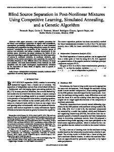
Validation of the asymptotic performance: Herein,

the evaluation of the domain of validity of the rst-order performance approximation (12) is considered. The previous settings are used with the exception of the source signals which are deterministic sinusoids at frequencies f1 = 0:4375 and f2 = 0:0625. The TFDs are computed using windowed Wigner distribution. The chosen window width is M = 2TL + 1, with L = 32. The identi cation is performed using M STFD matrices spaced in time by M samples (T being the sample size). The overall rejection level is evaluated over 500 independent runs. In Fig.1, the rejection level Iperf is plotted in dB as a function of the noise power 2 (also expressed in dB). In Fig.2, the rejection level Iperf is plotted in dB as against sample size. Both gures 1 and 2 show that the approximation is better at high SNR and for large sample size. This means that the asymptotic conditions are reached faster in this range of parameters.

T

X sp (t)sq (t) rT pq = T1 t=1 Jpq = (AH A)?pq1 +1 X Fsk;l = (m; v)(m ? v ? v0 + tk ? tl ;v0 ) p sp v ;v;m=?1 sp (tk + m + v)sp (tk + m ? v ? 2v0 )e?j4fk v e?j4fl v +1 X (m;v) (m + (tk ? tl );v)e?j4(fk ?fl )v kl = v;m=?1 For high signal to noise ratio, the expansion (12) is domi0 . Below, some comments on this nated by the rst term Ipq term are given: 0

0

1 We admit that a source separation algorithm fails when the mean rejection level is greater than ?10 dB.

3

Spectral shift (f )

0.000 0.002 0.010 0.050 0.200

7. CONCLUSION

In this paper, the problem of blind separation of linear spatial mixture of non-stationary source signal based on time frequency distributions has been investigated. A solution based on the diagonalization of a combined set of spatial time frequency distribution matrices has been proposed. A closed form expression for the performance criterion of the method has been developed. Numerical simulations have been provided to support the theoretical claims.

Mean Rejection level in dB SOBI TFS -8.86 -12.22 -10.01 -12.21 -10.18 -12.34 -11.09 -12.53 -12.92 -12.54

REFERENCES

Table 1. Performance of SOBI and TFS algorithms vs f

[1] C. Jutten and J. Herault, \Detection de grandeurs primitives dans un message composite par une architecture de calcul neuromimetrique en apprentissage non supervise," in Proc. Gretsi, (Nice), 1985. [2] P. Comon, \Independent component analysis, a new concept?," Signal Processing, vol. 36, pp. 287{314, 1994. [3] J.-F. Cardoso and A. Souloumiac, \An ecient technique for blind separation of complex sources," in Proc. IEEE SP Workshop on Higher-Order Stat., Lake Tahoe, USA, 1993. [4] A. Belouchrani and J.-F. Cardoso, \Maximum likelihood source separation for discrete sources," in Proc. EUSIPCO, pp. 768{771, 1994. [5] L. Tong and R. Liu, \Blind estimation of correlated source signals," in Proc. Asilomar conference, Nov. 1990. [6] A. Belouchrani and K. Abed Meraim and J.-F Cardoso and E. Moulines, \A blind source separationtechnique using second order statistics," IEEE Trans. on SP, 1996. To appear. [7] K. Matsuoka, M. Ohya and M. Kawamoto, \A neural net for blind separationof nonstationarysignals," Neural Networks, vol. 8, pp. 411{419, 1995. [8] L. Cohen, Time-frequency analysis. Prentice Hall, 1995. [9] J. Jeong and W. Williams, \Kernel design for reduced interference distributions," IEEE Trans. on SP, vol. 40, pp. 402{ 412, Feb. 1992. [10] R. Baraniuk and D. Jones, \A signal dependent timefrequency representation: Optimum kernel design," IEEE Trans. on SP, vol. 41, pp. 1589{1603, Apr. 1993. [11] G.H. Golub and C.F. Van Loan, Matrix computations. The Johns Hopkins University Press, 1989. [12] A. Belouchrani and M. G. Amin, \ Blind Source Separation Based on Time-Frequency Signal Representation.," IEEE Trans. on SP, 1996. Submitted.

−20 Sample size: 6500 − − : Experimental performance

−21

Mean rejection level in dB

− : Theoretic performance

−22

−23

−24

−25

−26 −30

−25

−20

−15 Noise level in dB

−10

−5

0

Figure 1. Performance validation vs 2 .

−10 Noise level: 5 dB − − : Experimental performance

−12

− : Theoretic performance Mean rejection level in dB

−14

−16

−18

−20

−22

−24 0

1000

2000

3000 4000 Samples

5000

6000

7000

Figure 2. Performance validation vs samples size (T).

4