Single Channel Blind Source Separation Using Independent ...

Single Channel Blind Source Separation Using Independent Subspace Analysis by

Jason Heeris

Submitted in partial fulfilment of the requirements for the degree of

Bachelor of Engineering

School of Electrical, Electronic and Computer Engineering The University of Western Australia

October, 2007

The Dean Faculty of Engineering Computing and Mathematics The University of Western Australia 35 Stirling Highway CRAWLEY WA 6009 Dear Sir, I submit to you this dissertation entitled “Single Channel Blind Source Separation Using Independent Subspace Analysis” in partial fulfilment of the requirement of the award of Bachelor of Engineering. Yours faithfully

Jason Heeris

Contents 1 Introduction 1.1 Motivation . . . . . . . . . . . . . . . . . . . . . . . . . . . . . . . . 1.2 Project Aims and Scope . . . . . . . . . . . . . . . . . . . . . . . .

1 1 2

2 Background 2.1 Single Channel Blind Source Separation . . . . . . . . . . . . . . . . 2.2 Independent Component Analysis . . . . . . . . . . . . . . . . . . . 2.3 Independent Subspace Analysis . . . . . . . . . . . . . . . . . . . .

3 3 5 6

3 Theory and Methodolody 9 3.1 Elements of Independent Subspace Analysis . . . . . . . . . . . . . 10 4 Implementation and Results 23 4.1 Implementation . . . . . . . . . . . . . . . . . . . . . . . . . . . . . 23 4.2 Overall Results . . . . . . . . . . . . . . . . . . . . . . . . . . . . . 24 5 Conclusion 33 5.1 Future Work . . . . . . . . . . . . . . . . . . . . . . . . . . . . . . . 34 A List of Symbols

37

i

ABSTRACT Single Channel Blind Source Separation Using Independent Subspace Analysis by Jason Heeris Supervisor: Dr. Roberto Togneri The problem of separating conceptually distinct sources of information in a single channel mixture signal, known as single channel blind source separation, was approached using the technique of independent subspace analysis, an extension of independent component analysis. A prototype system was implemented and tested in the numerical processing language Octave and showed reasonable success at separating simple test signals. The prototype failed to adequately separate mixtures of speech and noise, however, and its performance was severely degraded when adapted to operate on non-stationary signals. The inability to select an optimal level of detail to retain during processing coupled with the unsatisfactory non-stationary operation appear to be the main weaknesses of this technique, and further development should focus on improving these points.

Acknowledgements This project made heavy use of the numerical processing language and environment GNU Octave. This software is free and open-source, and I am sincerely grateful to all of the developers of the application and the various packages that accompany it for voluntarily producing free software of such quality. I would also like to acknowledge the authors of the Boston University Radio News Corpus, a comprehensively annotated database of human speech samples, and those of the noisex database. Both of these sources were used to test the prototype implemented for this project. Finally I would like to thank my supervisor, Dr. Roberto Togneri, for his help and guidance throughout this project.

v

Single Channel Blind Source Separation Using Independent Subspace Analysis

Chapter 1 Introduction Methods for extracting distinct streams of information from a single mixed signal have applications ranging from audio processing to astrophysics, and may not only find deployment in signal processing technology but could also form the basis for more sophisticated data analysis techniques. This problem is known as single channel blind source separation, and a number of methods have been used to solve it with varying degrees of success, based on learning algorithms, heuristics and programmed rules, or even the physics of the mixing process itself. The techniques differ substantially in their respective levels of applicability, robustness and computational efficiency. Successful though these methods are, they do have certain limitations on their effectiveness and on their scopes for applicability. This project focuses on one emerging method in particular: independent subspace analysis, a single channel blind source separation approach developed from the multi-channel analysis technique of independent component analysis. Independent subspace analysis (ISA) is a method which ideally requires little or no knowledge of the sources or the mixing mechanisms involved, working only on the inherent information content and spectral structure of the signal itself.

1.1

Motivation

The areas of audio processing and biomedical signal processing have been the motivation behind and the focus for much of the development of source extraction and filtering techniques, and are consequently the most likely areas of applications for a successful single channel source separation system. For example, this project was initiated in the context of speech filtering for voice recognition. It is possible that an effective implementation of ISA could be either used in isolation as a preprocessing tool, or be combined with another technique to improve performance Page 1

Single Channel Blind Source Separation Using Independent Subspace Analysis or simplify operation of a speech recognition system. The potential applications for a system like ISA is not just limited to the traditional areas already explored. One particularly interesting advantage of ISA is that the methods discussed above require a priori information about the sources of interest and therefore need either data suitable for training and analysis or detailed knowledge of the fundamental processes involved. This may be impractical or intractable, and in cases involving signals of unknown structure or composition even impossible. Independent subspace analysis, in theory, does not require knowledge of the signals it is required to separate and might therefore form the basis for novel techniques to analyse data to which other techniques are unable to be applied.

1.2

Project Aims and Scope

This project aims to investigate ISA as a technique for single channel blind source separation by implementing a prototype and examining its operation at various stages of processing. Overall, this project is looking not just for successful operation on simple signals but to evaluate whether ISA might eventually be viable for general applications requiring robust source separation techniques. Particular attention will be on how further investigations might be made easier or more successful, and to identify theoretical and practical weaknesses of the techniques with a view to narrowing the scope for future development. A review of current literature on, motivation for, and previous work in the area of single channel blind source separation is presented in Chapter 2. Expanding on this background, the theory behind ISA and its component stages is reviewed and discussed in Chapter 3. The implementation and demonstration of a prototype of an ISA-based system based on one particular implementation along with certain variations is detailed in Chapter 4, illustrated with results at intermediate stages. Chapter 4 also looks at the results of the prototype as applied to test signals to establish limits on the realistic expectations of the performance of ISA, as well application to some mixtures of audio signals, particularly speech. Finally, Chapter 5 will summarise the results, present the main outcomes of the investigation and discuss recommendations for further work.

Page 2


Chapter 2 Background 2.1

Single Channel Blind Source Separation

In the field of single channel blind source separation, some specific methods feature prominently because of their successful applications to certain types of signals. There are two classes of approaches that are particularly interesting in the context of this project due to their widespread use in signal processing in general, and because of their successes in the specific area of audio processing and speech filtering. These are learning algorithms known as support and relevance vector machines (SVM and RVM) and the heuristics-based computational auditory scene analysis (CASA) methods.

2.1.1

Computational Auditory Scene Analysis

Computational auditory scene analysis uses rules and heuristics based on the relevant physical processes it is attempting to emulate. In particular, human perception appears to operate (at a simple level) on proximity of dominant spectral features, and this behaviour can be used to build a CASA extraction algorithm. This technique almost exclusively focuses on attempting to replicate human psychoacoustic processing for speech extraction and signal separation. A comprehensive treatment of the emergence of CASA is given by Bregman[3]. Brown and Cooke show how to use this approach to construct a model which can separate speech from various types of noise and interfering signals[4]. They begin with filtering based on the modelling of the human ear, from the spectral response of the outer ear right through to the transduction of acoustic energy into nerve signals. This is followed by implementing an array of various filtering and processing stages intended to reproduce human physiological and psychoacoustic processes. Finally, the components which have been thus extracted are recombined according to rules based on spectral features significant to speech and hearing. Page 3

Single Channel Blind Source Separation Using Independent Subspace Analysis Van der Kouwe et al[24] implemented this technique and tested it against two implementations of independent component analysis (ICA is reviewed below). They found that the two techniques had different areas of effectiveness, with ICAbased techniques consistently performing better on statistically distinct signals than CASA. They also noted, however, that CASA was better suited to the separation of signals that depart from this condition of statistical independence, and that the combination of the two approaches might improve performance over the techniques being used in isolation. Although successful, CASA as a technique is not easily generalised. The effort required to implement an entire CASA algorithm for a new situation may be something of a drawback when compared to a method that should only require new training data or parameters to be adapted to a new application.

2.1.2

Classification Machines

An alternative to explicitly programmed rules is an algorithm that ‘learns’ the characteristics of the data it is required to extract. This type of approach is based around an algorithm that can give a binary classification of new input using a decision function. The decision function is constructed to contain adjustable parameters which are determined by a set of training data – examples of input that are each explicitly denoted as belonging to one set or the other. A classification machine can be used for speech filtering, for example, by being given a spectrogram of the signal and ‘deciding’ whether each cell of the spectrogram belongs to the speech source. Classification machines have an inherent trade-off between their accuracy and the number of parameters with which they operate, and making the wrong compromise may result in an inaccurate or computationally inefficient machine. The support vector training algorithm, outlined by Boser et al[2], is one solution to this problem and is based on automatically optimising the amount of information retained by a pattern classification function. This yields a pattern classification machine — the support vector machine (SVM) — that is best able to achieve accurate, non-trivial classification of new patterns. The tutorial on support vector machines by Burges[5] contains a detailed history of this method. The relevance vector machine has essentially the same functional structure as the SVM, but is based on a probabilistic approach to classification (as opposed to binary) put forth by Tipping[22, 23], who details the theory behind the RVM as well as a set of demonstration implementations and benchmarked tests against the SVM. The RVM algorithm is more computationally complex than the SVM, but makes up for this with the fact that less information needs to be retained by Page 4

Single Channel Blind Source Separation Using Independent Subspace Analysis the machine for the same (or greater) level of accuracy. Weiss and Ellis[25] found greater success using both RVM and SVM methods over CASA for extracting speech, also showing that there may be significant merit in combining the two methods. Essentially, the RVM and SVM must take training data in the form of signals that are characteristic or representative of the signals of interest, and are then able to extract this particular type of signal from mixtures. If such training data does not exist or is not comprehensive enough, or if a system might be expected to be used in unfamiliar situations, this technique becomes less useful and may not be applicable.

2.2

Independent Component Analysis

Independent subspace analysis, the focus of this project, is fundamentally an extension of independent component analysis (ICA), a widely-used method for demixing multi-channel signals. Independent component analysis operates on two fundamental assumptions: that the sources to be separated are statistically independent, and that there are as many sources (or fewer) as there are channels of data available. It can be considered a higher-order analogous technique to principal component analysis, which is used to decorrelate multi-dimensional data (further detail on PCA is covered by Jolliffe[16]). It is important to make the distinction between finding decorrelated variables (the aim of PCA) and independent variables (the aim of ICA), because it is possible for variables to be dependent but fail to be correlated. Decorrelation is essentially a second-order constraint on the statistical relationship between variables, while independence must be characterised by higher-order measures. Independent component analysis has been used extensively in biomedical signal processing as well as in imaging and audio processing[15]. Even economics and finance have seen ICA employed to reveal previously unidentified patterns in stock market data and form new predictors for economic performance[1]. Biomedical applications in particular have seen extensive successes of ICA as a data analysis technique because it is able produce signals that may be reliably compared between subjects, to separate signals of interest from other non-trivial noise and to identify components that may have physiological significance. Jung et al. review many applications of ICA in biomedical signal processing and elsewhere[17]. In electroencephalography (EEG) ICA has been used to remove noise associated with irrelevant physical processes (such as blinking) and identify functionally distinct components and statistics which can be meaningfully compared between experiments. It has also been applied to electrocardiography (ECG/EKG), for Page 5

Single Channel Blind Source Separation Using Independent Subspace Analysis example in the separation of maternal and foetal ECG signals by De Lathauwer et al[10]. It was this particular application which inspired the generalisation of the ICA theory to the extraction of multi-dimensional sources as formalised by Cardoso[6], giving rise to the theory of independent subspace analysis. Independent component analysis can be performed using a variety of algorithms and constraints but ultimately has a single unifying foundation in information theory. This is demonstrated by Lee, et al.[20], who tie together many of the different theoretical bases and algorithms used for ICA, proving their equivalence and developing a framework for further development. An excellent overview of the ICA methodology is also given by Hyv¨arinen[14] who discusses not just the theory behind its various components but some of the practical implementations available and their constraints and limitations.

2.3

Independent Subspace Analysis

Although ICA has proven useful in the fields already discussed, it suffers from one — often intractable — drawback. Independent component analysis works on the assumption that there are at least as many channels as sources, and in many practical situations this assumption is just not valid. Although this restriction has been worked around in some applications, in the case of a single channel of data it would seem that ICA is simply unable to be used. In actual fact, applying ICA to single channel audio signals forms part of the statistical and group theoretic audio analysis framework presented in a PhD thesis by Casey[8]. In this thesis, Casey develops powerful techniques for decomposition of audio signals into components suitable for ICA and then for further, abstract analysis (such as music classification). The extracted components, however, were not necessarily conceptually meaningful signals (such as the musical instruments themselves), and so the applicability of these techniques was limited to areas only requiring characterisation of signals rather than their actual separation. Casey and Westner applied independent subspace analysis to audio separation in 2001[9], connecting the audio processing techniques from Casey’s thesis with multi-dimensional ICA (mentioned above) to create a method that would work on single channel mixtures. Their paper details the various components of ISA — particularly the clustering method used to reconstruct sources — and demonstrates the method successfully operating on noisy speech and synthesised music. Most of the development and application of ISA to single channel analysis has been in the area of computer music processing, a field which is almost universally restricted to analyse signals with far fewer channels available than the amount of information required. One such application of ISA is documented in a PhD Page 6

Single Channel Blind Source Separation Using Independent Subspace Analysis thesis by Orife[21], where ISA forms an integral part of a music analysis software suite. Orife uses ISA to detect rhythm from the temporal structure of the extracted components, also demonstrating the utility of using ISA to support other methods by combining it with heuristics. Another example is a sub-band adaptation of ISA for analysing drum mixtures by FitzGerald et al[11]. In this paper, some of the limitations of ISA are discussed with some possible solutions, including modelling of the sources and filtering at the intermediate stages of analysis. An important aspect of applying ISA to the area of music analysis is that it is not strictly necessary to separate the actual (conceptual) sources encapsulated by a music track (ie. the individual instruments) in order to achieve typical objectives of, say, music classification or melody identification. For example, it may be enough to just quantify the presence of characteristic frequency bands. This is something achievable by ISA but is in distinct contrast to the focus of this project, which is to evaluate the suitability of ISA for separation of the actual sources of interest. With classification machines and CASA being relatively successful, an important question is whether it would be more rewarding to pursue these avenues of enquiry in the first place. Independent subspace analysis was chosen as the focus of the project because, in theory, it appears to be a promising technique for the area of single channel blind source separation yet has seen little real testing or demonstration in this area. Despite the successful applications of ISA discussed above, there is little quantitative evaluation of ISA as a source separation method and no literature could be found that compared ISA to other techniques. While some qualitative and quantitative comparisons have been made between unrelated approaches and other ICA-based methods, none have been found which avoid the constraint of requiring multiple channels of data. The classes of separation techniques discussed earlier — CASA and classification machines — are much more established and researched than independent subspace analysis, and so it is difficult to evaluate the true value of the theoretical advantages apparent in ISA over SVM, RVM or CASA without a working ISA prototype. This forms part of the basis for this project: not so much to create a working ISA system all at once, but to identify the potential that this technique might have and to establish possible direction for future work. The primary aim of this project is to develop a ISA-based prototype which can be applied to single channel time series data (particularly audio signals), to evaluate its performance and to identify its weaknesses. Ultimately, this will enable the appraisal of the potential for ISA to be developed to a point suitable for applications requiring robust single Page 7

Single Channel Blind Source Separation Using Independent Subspace Analysis channel blind source separation. Another reason to examine ISA is the possibility of areas of application that are not currently known. Just as CASA and classification machines have complementary domains of effectiveness, ISA may be found to be useful for areas not already explored by these approaches. The theory behind independent subspace analysis encompasses information theory, statistics and signal processing, and it may well be the case that further research into ISA reveals new ways to analyse information, even if ISA itself is ultimately deemed unsuitable for blind source separation. The most ambitious prospect for an ISA-based signal processing system is in applications to fields of research that would benefit from novel single channel analysis methods, but which cannot exploit the methods currently available. Independent subspace analysis may be a valuable tool in areas which cannot use trained extraction methods due to a lack of data, or which cannot use heuristics due to lack of knowledge. In an analogous way to ICA revealing hidden patterns in economic and financial data, ISA may be able to be used to discover new aspects of data that other approaches might miss completely, and it is this potential which is one part of the motivation for further investigation and development.

Page 8


Chapter 3 Theory and Methodolody The fundamental problem of single channel blind source separation is that we have a single stream of data comprising several different sources, and we wish to extract one or all of the sources from the mixture given as little extra information as possible. These sources could be physically separated in space such as voices in a room, or the distinction could be conceptual such as instruments in synthesised music. This chapter will outline exactly how independent subspace analysis can be used to solve this problem, detailing the important components of the prototype to implemented. Formally, the problem to be solved by the prototype is as follows: we are given a single channel signal consisting of data sampled with a frequency of fs , which can be represented as a column vector x with N components:    x=  

x (t1 = 0) x (t2 ) .. .

     

x (tN ) This signal is known to represent a mixture of several different signals yλ , so that κ X x= yλ λ=1

Note that this expression contains some implicit assumptions about the mixing mechanism: that it is linear and involves no convolution of the sources with another process (such as would be introduced by, say, echoing). The objective is then to estimate the source signals (yλ ) as closely as possible, perhaps given the number of sources known (κ). This problem is clearly underdetermined, and the additional information required to solve it comes in the form of the assumption that the sources producing the signals yλ are statistically Page 9

Single Channel Blind Source Separation Using Independent Subspace Analysis independent. This assumption enables the use of independent component analysis and certain clustering techniques based on information theoretic measures of independence. Since this project is undertaken primarily in the context of cleaning speech signals for voice recognition, most of the analysis will be discussed in the context of audio processing.

3.1

Elements of Independent Subspace Analysis

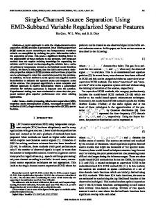
Independent subspace analysis is a single-channel extraction method built around the multi-channel analysis technique of independent component analysis. In order to utilise ICA for the problem of single-channel blind source separation, there must be a way to produce enough input signals upon which ICA can properly operate, and some way to combine the multitude of ICA output signals into contrasting signals. Furthermore, the signals which are passed to ICA must be of the appropriate form to achieve the goal of extracting maximally contrasting features, and the method used to group components must be reliable enough to construct meaningful sources based on the ICA output. The overall method is illustrated in Figure 3.1, and essentially involves forming subspaces that each represent a particular source. The subspaces comprise statistically independent signals which represent spectral features of that source, meaning that the original signal can be projected on to the subspaces to extract the source — the ultimate output of the prototype.

3.1.1

Spectrogram Decomposition

Before applying ICA, the original single channel signal must be decomposed into a set of signals suitable for analysis. This is achieved by using principal component analysis, which can be performed by finding the singular value decomposition of the spectrogram of the signal[16]. We can then select vectors which sufficiently represent a specified proportion of information in the signal. The original signal x is split into m frames of length w. These frames are arranged into a w × m matrix X (note that no window function is applied1 ) which can then be multiplied by a matrix T (l × w) representing a linear transform to obtain the spectrogram S = T X. This transform is (for the scope of this project) taken to be square, and may be any linear or otherwise invertible transform — most often used is the Fourier transform. Note that the spectrogram used for 1

Although using a rectangular (boxcar ) window causes aliasing problems in the spectrogram, using a more sophisticated window creates problems when inverting the transform.

Page 10


Figure 3.1: Schematic of ISA prototype implementation. The original signal can be projected on to the subspaces to recover the separated sources.

further calculations is still complex-valued.

The spectrogram S is then subjected to singular value decomposition (SVD), where it is factorised as S = U ΣV H

where U and V are unitary matrices (l × l and m × m) and Σ is a diagonal Page 11

Single Channel Blind Source Separation Using Independent Subspace Analysis l × m matrix containing the singular values of S in descending order, so that2    Σ=  

σ1 0 · · · 0 0 σ2 · · · 0 .. .. . . . 0 . . 0 0 0 σn

     

with σi ≤ σi+1

Informally, the application of SVD to the spectrogram extracts spectral features that form a basis for column or row space of S, which are ranked in order of prominence by the singular values. The matrix U contains a basis for S to be expressed as time varying weights of a set of spectra, while the matrix V can be used to express S as a set of temporal features with weights varying across the frequency bands. The singular vectors will in fact have distributions closer to Gaussian than any other basis for the spectrogram, and therefore the least contrast (ie. highest mutual information) with each other[8]. This can be taken to mean that in selecting a certain number of vectors, we are selecting a proportion of information to retain for further analysis. This can be specified by the information ratio[9] φ ∈ [0, 1] using !−1 ρ n X X φ= σi σi (3.1) i=1

i=1

This expression defines ρ, the number of signals to pass to ICA. The value of the information ratio has a significant impact on the performance of the prototype. It is worth noting that if the signal is simply reconstructed from the principal components retained from SVD (ie. skipping the further stages of operation), there will be noticeable degradation — a problem which gets worse as the information ratio decreases and more detail is discarded. However, if the information ratio is too high then the independent components will be compact frequency bands too difficult to group, and the sources will not be properly separated. This means that if the remaining stages of the prototype fail to faithfully reconstruct the source signals as required, the output will be noisier than the input and the model will become a hindrance to any system in which it is deployed. This is clearly a fatal drawback, but one which this project was unable to solve. Figure 3.2 illustrates the relationship between the number of singular vectors and the information ratio for a spectrogram (50ms boxcar windowed Fourier transform) of a mixture of speech and machine gun noise. For normal applications, an information ratio of 0.7 to 0.8 is usually selected — although there is no known way to systematically find the optimal value for φ. This is a significant weakness 2

Page 12

Note that Σ may have extra rows or columns of zeros, depending on l and m.

Single Channel Blind Source Separation Using Independent Subspace Analysis 1

Information ratio

0.8

0.6

0.4

0.2

0 0

100

200

300

400

500

Index

Figure 3.2: Normalised, cumulative sum of singular values for the spectrogram of a 26s mixture of speech and machine gun noise. An information ratio of 0 .8 yields 96 basis vectors.

of the prototype given the high sensitivity of the quality of the output to this single parameter. With no easy way to determine the information ratio prior to processing, this severely limits not only the practicality of the method but the ability to investigate it thoroughly in the first place. At this point, there are some variations on how obtain suitable input for the next stage (independent component analysis). This is where one particular property of the Fourier transform becomes immediately relevant: the spectral symmetry of real signals. Briefly, when a signal consisting of only real values is subjected to the Fourier transform, one side of the spectrum is effectively a copy of the other half — the real components of the spectrum are symmetric about the frequency origin, and the imaginary components are antisymmetric. This means that the ‘upper half’ (ie. the first half of the rows) of a spectrogram have exactly this symmetry with the lower half. This is noteworthy here because it is possible to perform ICA on the first ρ vectors of either the frequency bases from U or the time bases from V . If ICA is performed on U , however, it will destroy the symmetry of the phase information which will need to be reconstructed somehow. One way around this is to exploit this symmetry and keep only one half of the rows of S — discarding the redundant information arising from performing a Fourier transform on a real signal. This new ‘folded’ matrix can then be decomposed used SVD, and the eventual output of ICA can then be ‘unfolded’ so that real signals are recovered. Another way to avoid this is to perform analysis only on the magnitude spectrum of x (ie. on |S|). This results in the complete loss of phase information, Page 13

Single Channel Blind Source Separation Using Independent Subspace Analysis however, and subsequent corruption of the recovered signals. It also affects the reliability of the clustering stage (for reasons explained in Subsection 3.1.3 on clustering). One variation explored by Orife[21] for identifying onset of features in music analysis uses the auto-correlation matrix of the spectrogram for SVD and performs ICA on the time-varying weightings rather than the signals themselves. This method was implemented but showed little success on simple test signals or realistic mixtures. The method used for this project takes the first ρ columns of V (vectors of length m, the number of frames) for ICA. This approach shows the most success on simple test signals (for example, those in Figure 4.1), and is the de-facto implementation discussed in the results section. Its drawback is that instead of producing signals of length w (as would be possible using vectors from U ) it produces signals of length N (the original length of the signal), making it computationally intensive when using the stationary model of ISA. It can still be used for the non-stationary extension of the prototype (see subsection 3.1.4), since the spectrograms formed are the size of the much shorter signal blocks, rather than the entire signal.

3.1.2

Independent Component Analysis

The singular value decomposition produces minimally contrasting signals that represent mixtures of independent features of the source spectrogram. Independent component analysis is the next step, and forms the conceptual core of independent subspace analysis. The idea behind ICA is that we have a mixture (the vi ) of statistically independent signals (the bi )3 :      

v10 v20 .. . vρ0





     = A    

b01 b02 .. . b0ρ

     

and our objective is to find the mixing matrix A to be able to recover the independent signals. A popular example of an ICA problem is the ‘cocktail party problem’: given a room full of people speaking, and given as many microphones as people placed in various locations throughout the room, the goal is to reproduce the unmixed signals of each person’s speech. A variety of algorithms can be employed to achieve this, but the result should be the same: a set of signals whose probability densities are as dissimilar as 3

Page 14

Note the expression uses the signals in rows, for consistency with other literature.

Single Channel Blind Source Separation Using Independent Subspace Analysis possible. Figures 3.3 and 3.4 show ICA operating on mixtures of some simple test signals obtained from the FastICA package (Jade was used for analysis in this case, but all implementations worked just as well). Note that the output of ICA was originally in a different order and had some signals inverted, but for ease of comparison they were reordered and flipped (but not rescaled). Independent component analysis will, in theory, extract the independent features from the SVD signals which can then be grouped into the conceptual sources. In practice, however, independent component analysis has trouble when one of the original signals (ie. the desired output) is close to Gaussian — as is the case not only with common forms of noise but with many realistic signals such as specific forms of music. Once these signals are recovered, a set of corresponding spectrograms can be recovered by projecting S onto the the vector bi . If the signals used are from V (of length m), these spectrograms can be recovered by computing

Si =

0 (bi )+ S 0 b0i

or Si = (S/b0i ) b0i where X + is the pseudo-inverse of the matrix X (or, in this case, the vector). If the signals used form frequency bases (from U , of length l), these spectrograms can be recovered by computing

Si = bi b+ i S

or Si = bi (bi \S) These spectrograms can then be inverse-transformed into signals (the xi ) which form the basis components of the subspaces to be constructed.

3.1.3

Subspace Grouping

Applying ICA to the set of vectors from SVD yields a set of ρ independent basis signals, which must be grouped into subspaces in order to reconstruct the individual sources. The goal is to now reconstruct the most independent sources possible given the basis signals from ICA. As mentioned earlier, one way to measure the independence of two random variables is to compare their probability distributions, and this can be done using the Kullback-Leibler (KL) divergence, which operates Page 15


2

3

2

0

0

0

-2

-3

-2

4

4

4

0

0

0

-4

-4

-4

3

6

3

0

0

0

-3

-6

-3

4

2

4

0

0

0

-2

-4 0

50

100

150

200

-4 0

250

(a) Original signals

50

100 150 Samples

200

250

0

50

(b) Random mixtures

100

150

200

250

(c) ICA output

Figure 3.3: Demonstration of ICA applied to simple test signals

Sinusoid

Sawtooth

1

0.5

0.8

0.4

0.6

0.3

0.4

0.2

0.2

0.1

0

0 -4

-3

-2

-1

0

1

2

3

4

-4

-3

-2

-1

0

1

2

3

4

3.5

0.6

3

0.5

2.5

0.4

2 0.3 1.5 0.2

1

0.1

0.5 0

0 -4

-3

-2

-1

0 1 Quintic

2

3

4

-4

-3

-2

-1 0 1 Skewed Random

2

Figure 3.4: Histograms and ideal probability densities for the signals in Figure 3.3.

Page 16

3

4

Single Channel Blind Source Separation Using Independent Subspace Analysis 0

0

5

5

5

10

10

10

15

15

15

20

20

20

25

25

25

30

30

30

35

35

35

40

40

40

45

45 0

5 10 15 20 25 30 35 40 45

(a) Ixegram of principal components (ie. before ICA)

0

45 0

5 10 15 20 25 30 35 40 45

0

(b) Ixegram of independent components

5 10 15 20 25 30 35 40 45

(c) Ixegrams of independent components, grouped into two subspaces

Figure 3.5: Ixegrams (dissimilarity matrices) of component vectors extracted from speech and factory noise. Lighter points indicate greater similarity.

on two probability densities p(u) and q(u):

Z δKR (p, q) =

p(u) log dom(u)

p(u) q(u)

du

(3.2)

This divergence measure is not symmetric, but can symmetrised trivially by using 1 δSYM (p, q) = (δKR (p, q) + δKR (q, p)) (3.3) 2 Where only a finite number of realisations are available, the densities can be approximated by the histograms. Unfortunately, histogram approximations show sensitivity to bin width and centre, and cause the KL divergence to become highly sensitive to small variations between density functions. Other methods were investigated for approximating density functions from finite realisations, such as the Edgeworth or Butterworth expansions. These approximations use the cumulants (the unbiased estimators for which are the k -statistics) and express the density function as a perturbation from a Gaussian distribution. These proved unsatisfactory, however, often producing divergent approximations or invalid density functions, especially when applied to sharp densities such as that of speech (both are known weaknesses of these expansions[18]). In order to apply a clustering algorithm, we must have either an external Euclidean space in which we can compare each signal or some pairwise similarity or distance measure. Following the methodology of Casey and Westner, the symmetric Kullback-Leibler divergence is used as a pairwise measure to create a dissimilarity matrix which can be used to group the components based on this measure. The ρ × ρ independent component cross-entropy matrix (ixegram) D is formed Page 17

Single Channel Blind Source Separation Using Independent Subspace Analysis by calculating the KL divergence for each possible pair of signals. Interestingly, the matrix thus formed actually provides a simple, graphical explanation to illustrate independent component analysis: the goal of ICA is equivalent to maximising the contrast of the ixegram — compare Figures 3.5(a) and 3.5(b). The entries in the ixegram form a suitable pairwise distance measure for the deterministic annealing clustering algorithm outlined by Hofmann and Buhmann[12], where the grouping of the signals is represented by a ρ × κ assignment matrix M , defined by 

P (x1 ∈ Y1 ) P (x1 ∈ Y2 )   P (x2 ∈ Y1 ) P (x2 ∈ Y2 ) M =  .. ..  . .  P (xρ ∈ Y1 ) P (xρ ∈ Y2 )

· · · P (x1 ∈ Yκ ) · · · P (x2 ∈ Yκ ) .. .. . . · · · P (xρ ∈ Yκ )

     

with the restrictions Miλ ∈ {0, 1}

and

κ X

Miλ = 1

λ=1

That is, assignments are binary, exhaustive and exclusive. A cost function H (M | D) measures the favourability of a particular allocation given the pairwise distance matrix D, based on similarity within clusters and contrast between clusters: ! ρ ρ κ 1 X X Dij X Miλ Mkλ −1 (3.4) H (M | D) = 2 i=1 j=1 ρ pλ λ=1 ρ

where pλ

1X = Miλ ρ i=1

The problem of grouping then becomes finding the binary matrix M that will minimise the cost function H. To approach this using deterministic annealing, Hofmann and Buhmann define mean-field potentials εiλ which are related to the expectation values hMiλ i of the assignments4 . The system is minimised by defining a Lagrangian parameter T (known as the temperature for the statistical mechanics analogy). At the optimal solution for a given ‘temperature,’ T , the potentials and

4

Note that the hMij i, being expectation values, are not restricted to take only the values {0, 1}.

Page 18

Single Channel Blind Source Separation Using Independent Subspace Analysis assignment expectations satisfy ε?iλ = Pρ

j=1 j6=i

×

ρ X

1 hMjλ i + 1 

(3.5)

1 hMkλ i Dik − Pρ 2 j=1 hMjλ i k=1 j6=i

hMiλ i =

ρ X

 hMjλ i Djk 

j=1

exp (−ε?iλ /T ) Pκ ? exp −ε /T iµ µ=1

(3.6)

For any given temperature, these ρ×κ equations can be satisfied simultaneously by fixed-point iteration. At a high temperature, all local minima of the solution become degenerate and the assignment expectations tend to uniformity. As the temperature is lowered, the solutions to Equations 3.5 and 3.6 should converge to the global minimum of Equation 3.4, with the expectation values hMiλ i converging to the binary values Miλ as required. It should be noted, however, that this method is not guaranteed to converge to the global minimum in every situation, and is especially prone to failure when there is little contrast (in “cost”) between different clustering configurations. Ideally, this will classify the basis signals with the most similar probability densities (based on the KL divergence) into the same group, while maximising the difference between the groups (compare Figures 3.5(b) and 3.5(c), or Figure 4.3(a)). Since the grouping is based entirely on the difference in information between the independent components, the subspaces thus formed should be most distinct in terms of mutual information. The original signal can then be projected onto the subspaces to extract each source, which should be statistically independent from each other because the basis signals are all independent.

3.1.4

Extending ISA for Non-stationary Signals

The method outlined thus far operates in the context of a signal with stationary statistical properties. Casey and Westner demonstrated a straightforward method by which it is adapted to the non-stationary case under the assumption that the sources are approximately stationary for some specified short period of time (some multiple of the spectrogram window). The original signal is split into smaller signals of this length (which may overlap) and the preceding method is applied to each signal section. This will result in groups of separated signals which need to be allocated across adjacent time sections. This is achieved using an exhaustive search over all possible sets of pairings to minimise the cost using the same distance measure as per clustering. Page 19

Single Channel Blind Source Separation Using Independent Subspace Analysis This extension is not without its drawbacks, though: by reducing the length of the signal being passed as the input to the prototype, the spectrogram will have far fewer columns. The decreased size of the spectrogram means fewer SVD signals can be extracted, and the same information ratio will result in fewer component signals. This not only results in lower subspace resolution in the decomposition of the spectrogram, but decreases the ability of the deterministic annealing clustering algorithm to find the optimal grouping of the components which, in turn, decreases the accuracy of the method used to join subspaces across time sections. Thus applying the non-stationary version of ISA to a statistically stationary signal may actually result in a degradation in performance over the stationary model and produce non-stationary output signals. One possible solution to this problem is to establish an automated way by which the non-stationarity of an input signal may be detected and quantified in order to set the window and overlap for non-stationary ISA operation. This level of automation was deemed beyond the scope of this project, and investigations were restricted simply to manual selections of these parameters.

3.1.5

Theoretical Limitations

The separation technique outlined thus far relies on the statistical independence of the signals we wish to separate. It is reasonable to expect that if the source signals have very similar probability distributions then they may prove difficult or impossible to separate. This is a realistic possibility — for example, separating speech from babble noise, or separating similar musical instruments. An even more intractable manifestation of this limitation would be found in multipath noise (such as echoing), because it is essentially the replication of the original signal and should therefore show little or even no statistical contrast. Furthermore, the assumption of statistical independence of the sources is technically valid in most practical situations but its utility is questionable in many instances. Figure 3.6 on the facing page compares the histograms of music, speech, machine gun noise and factory noise. Although their densities are clearly distinct, the ability to quantify this difference reliably — especially for small samples, and in mixtures — is certainly one of the weaknesses of the prototype. While the KL divergence in Equation 3.3 is theoretically sound, the integrand is very sensitive to the inaccuracies introduced by histogram representation (or, for that matter, expansion approximation). Informally, the prototype will perform less effectively as the source signals become less distinct – an expected limitation of attempting to extract contrasting features of a signal.

Page 20


Factory noise

Speech

0.5

3

0.4 2 0.3 0.2 1 0.1 0

0 -4

-3

-2

-1

0

1

2

3

4

-3

-2

-1

0

1

2

3

18

2

15 1.5 12 9

1

6 0.5 3 0

0 -1

-0.5

0 0.5 Machine gun noise

1

-4

-3

-2

-1

0 Music

1

2

3

4

Figure 3.6: Histograms of various types of sound, all with unit power.

Page 21


Chapter 4 Implementation and Results The components and theory detailed in Chapter 3 form the basis for the prototype constructed in this chapter, which will be used to demonstrate the performance of ISA as a single channel blind source separation technique. Ideally, the input to this prototype would the single channel signal requiring separation, and the outputs should be the extracted sources. Realistically, at this stage of development it is also necessary to specify certain other parameters such as the number of sources to be separated, the transform window size and the amount of detail to retain. It should be noted that the idea of meaningful output is rarely able to be objectively determined, which means that it is usually not possible to automatically determine the number of sources to attempt to separate even in realistic situations. For example, in separating a piece of music comprising a few different instruments, it might be considered obvious from context that the goal is to separate the instrument tracks. Consider though an audio signal containing the same piece of music and some unrelated speech – it is no longer clear whether the goal might be separation into music and voice or to separate the instruments themselves and clean the speech signal. Despite the fact that this means that the prototype itself is not unsupervised, the variation of its internal parameters forms an important part of the evaluation of its performance and its sensitivity to these parameters.

4.1

Implementation

A prototype of an ISA system was implemented using the GNU Octave numerical processing language1 . Most components described above were written for this project with the exception of the ICA stage and auxiliary packages for signal processing, audio processing, imaging and plotting, and statistics. A variety of 1

The syntax and API is similar to Mathworks’ MatLab.

Page 23

Single Channel Blind Source Separation Using Independent Subspace Analysis ICA packages are available for use in Octave – the packages used for this project include FastICA[13], Jade[7] and RadICAl[19]. Of these, Jade is of particular interest as it can be applied to complex signals and therefore used in the frequency domain as well as the time domain.

4.2

Overall Results

Before attempting to apply ISA directly to realistic signals, it is instructive to use a mixture of some simple signals to demonstrate the processes involved. The signals used for testing are similar to those used to illustrate ICA in Figure 3.3 and are specifically formulated to have large statistical contrast. This means these signals should exhibit the best-case performance of ISA and illustrate the limit of what can be realistically expected from the prototype as it stands. Figure 4.1 shows sections of the time series form of a periodic quintic curve and a sawtooth wave used as test signals, along with histograms of their amplitude, a section of the time series form of their mixture (note the aperiodicity) and a spectrogram of the full mixture signal. The resulting mixture is passed to the ISA prototype and Figure 4.2 shows some important results at various intermediate stages of processing. Figure 4.2(a) shows the relationship between the information ratio φ and the number of basis components ρ (defined in Equation 3.1) for these signals. To attempt to find the optimal value of φ, the prototype was run for the minimal range of ρ (01 to 49) that that corresponded to the full range of φ ∈ [0, 1], and Figures 4.2(b) and 4.2(c) show the signal to noise ratio and KL divergence (scaled by the divergence of the original signals) for each value. The SNR for the input mixture was 0 dB for both signals. There are two important points that these graphs omit. Firstly, for values of ρ > 49 there was still some variation in the output signal SNR and divergences, due to the variations in the reconstructed signals using a different set of independent components. These fluctuations were deemed to have no real significance in evaluating the sensitivity of the prototype to φ or ρ, since the new components effectively contained no new information. The second point is that for values of ρ < 6 these measures were far lower than all subsequent values, indicating an effective ‘floor’ on the performance of the prototype, and were therefore omitted from the graph. Two things that are apparent from these graphs are the similarity between the SNR and KL divergence for values of ρ greater than about 30, which indicates that both are reasonable (although not necessarily the best) measures of merit. below this value, though, the KL divergence shows high variation despite inspection Page 24


3

3

0

0

-3

0

0.01 Time (s)

0.02

0

0.01 Time (s)

Amplitude

Amplitude

Figure 4.1: Input signals for ISA concept demonstration (quintic and sawtooth waveforms)

-3

0.02

(a) Component quintic (left) and sawtooth (right) signals (both of unit power) 3

0.4

Density

0.2 1

Density

0.3

2

0.1

0

0 -3

-2

-1

0

1

2

3

-3

-2

-1

0

1

2

3

(b) Histogram of quintic (left) and sawtooth (right) test signals

Amplitude

3

0

-3

0

0.01

0.02

0.03

0.04

0.05

Time (s)

(c) Superposition of above component signals 8

0

7 -10

-20

5 4

-30

3

Volume (dB)

Frequency (kHz)

6

-40

2 -50

1 0

-60 0

2

4

6

8

10 Time (s)

12

14

16

18

20

(d) Normalised spectrogram of mixture signal (50ms boxcar window)

Page 25

Single Channel Blind Source Separation Using Independent Subspace Analysis revealing no noticeable change in output quality. The maximum SNR for the output signals appears to occur at ρ = 48, which corresponds to φ = 1. The value of ρ (and therefore φ) was chosen to be 39 (0.92) to demonstrate non-trivial operation while still looking at near-optimal performance. Because of the high contrast of these signals, the optimal information ratio will certainly be much higher than for a mixture with less contrast, because the vectors passed to ICA will already have a higher degree of independence than for more Gaussian signals. This is also a result of the original signals having relatively compact presence in the frequency domain. Figure 4.3 shows the results for an information ratio of 0.92. It is interesting to compare the contrast inherent in these basis signals (Figure 4.3(a)) to those illustrated in Figure 3.5. The reconstructed test signals are shown in Figure 4.3(b). While they clearly resemble the shape of the original signals, a better basis for evaluating the separation of the signals are the histograms in Figure 4.3(c), where we see some degradation compared to the original histograms in Figure 4.1(a). These results indicate some degree of success, but it should be noted that this does not necessarily confirm the suitability of ISA as a technique suitable for realistic signals, which will certainly be less distinct and comprise mixtures of more sources. The next stage of this investigation was to apply the prototype to the separation of more realistic signals. Of course, it should be noted that ‘mixtures of realistic signals’ is not the same as ‘realistic signals’, but for the purposes of testing it is better to start with controllable sources that can be easily characterised. A variety of mixtures were used to test the prototype, including mixtures of speech2 , Gaussian noise, factory noise, traffic noise3 , music and pure tones. The outcome of all mixtures trialled, however, was the same: the prototype failed to separate the sources to any real extent, and always caused significant degradation of the signals themselves. Figure 4.4 shows the source signals for one such test: a mixture of machine gun noise and male speech. There is no significant difference between this mixture and any other tested – they were chosen because speech is relevant to the context of this project, and the machine gun noise is easier to present visually. These sources were scaled to unit power and combined to form the input signal to the non-stationary ISA prototype. Figure 4.4(c) shows the spectrogram of this mixture. Both the stationary and the non-stationary prototype struggled to separate this mixture, as the results in Figure 4.5 (for the non-stationary prototype) clearly 2

All speech samples were taken from a CD-ROM database of the Boston University Radio News Corpus. 3 Noise samples obtained from the NOISEX database.

Page 26


Figure 4.2: Effect of the information ratio φ on the performance of the ISA prototype for signals in Figure 4.1 1

Information ratio

0.8

0.6

1

0.4

0.2 400 0 0

10

20

30

40

50

Index

(a) Normalised, cumulative sum of singular values for spectrogram decomposition of test signals (first 50 singular values). An information ratio of φ = 92 gives ρ = 39 basis signals. Inset is graph of all 400 singular values.

SNR (dB)

40 30

Sawtooth Quintic

20 10 0 -10 10

15

20 25 30 35 Principal components

40

45

Relative KL divergence

(b) The signal-to-noise ratio of the two test signals in the prototype output signals as a function of ρ

12 10 8 6 4 2 0 10

15

20 25 30 35 Principal components

40

45

(c) Kullback-Leibler divergence of prototype outputs (scaled by unmixed divergence)

Page 27


Figure 4.3: Intermediate results and final output for ISA prototype with information ratio φ = 0.8 0

0

5

5

10

10

15

15

20

20

25

25

30

30

35

35 0

5

10 15 20 25 30 35

0

5

10 15 20 25 30 35

Amplitude

(a) Ixegrams for ICA output signals: unordered (left) and clustered into two subspaces (right). Lighter points indicate greater similarity. 3

3

0

0

-3 0

0.01 Time (s)

0.02

0

0.01 Time (s)

-3 0.02

(b) Extracted signals using stationary ISA constrained to two sources 0.5

1.2

0.3 0.2

0.4

Density

Density

0.4 0.8

0.1 0

0 -3

-2

-1

0

1

2

3

-3

-2

-1

0

1

2

3

(c) Histogram of ISA output signals 0.4 0.3

2

0.2 1

0.1

0

0 -3

-2

-1

0

1

2

3

-3

-2

-1

0

1

(d) Histograms of original signals (repeated for comparison).

Page 28

2

3

Density

Density

3


8

8

6

6

4

4

2

2

0 0

5

10

15 Time (s)

20

25

0

5

10

15 Time (s)

20

Frequency (kHz)

Frequency (kHz)

Figure 4.4: Mixture of speech and machine gun noise for realistic ISA demonstration

0 25

(a) Spectrograms of speech (left) and machine gun noise (right) (50ms boxcar window)

2

20

1

10

Density

30

Density

3

0 -1.5

0 -1

-0.5

0 0.5 Amplitude

1

1.5

-1.5

-1

-0.5

0 0.5 Amplitude

1

1.5

8

0

7

-10

6

-20

5

-30

4

-40

3

-50

2

-60

1

-70

0

Volume (dB)

Frequency (kHz)

(b) Histogram of above signals (speech, left, and machine gun noise, right)

-80 0

5

10

15

20

25

Time (s)

(c) Spectrogram of speech and machine gun noise mixture (50ms boxcar window)

Page 29

8

8

6

6

4

4

2

2

0

Frequency (kHz)

Frequency (kHz)


0 0

5

10

15 Time (s)

20

25

0

5

10

15 Time (s)

20

25

80

80

70

70

60

60

50

50

40

40

30

30

20

20

10

10

0 -0.15

-0.1

-0.05

0 0.05 Amplitude

0.1

0.15

-0.15

-0.1

-0.05

0 0.05 Amplitude

0.1

Density

Density

(d) Spectrogram of ISA output signals (50ms boxcar window)

0 0.15

(e) Histograms of ISA output signals

Figure 4.5: Results of non-stationary ISA on mixture of speech and machine gun noise

indicate. Although the output signals were not actually identical, they were in no practical way distinct and were far from representative of the original source signals. Furthermore, the quality of the output signals was not only far lower than that of the input signals, but even of the mixture itself – in other words, the output signals were also equal mixtures of both sources, but severely degraded. This means that another system needing clean input (for example, a voice recognition system) would almost certainly have better success on the original mixture than on the output of the prototype, completely defeating the utility of having an ISA based signal processing system. The details of operation of the non-stationary version of the prototype also showed some expected limitations — specifically that inadequate detail was retained from principal component analysis for effective clustering in the later stages of the process. For a window size of 50ms, a block size of 1.25s will produce spectrograms with 25 time frames, and typically only 5 − 10 principal components will be retained using an information ratio of 0.7 − 0.8. As mentioned previously, the deterministic annealing algorithm used for clustering is prone to failure when the ixegram has low contrast or is quite small (but still not small enough for exhaustive Page 30

Single Channel Blind Source Separation Using Independent Subspace Analysis searches). The information ratio, despite being the focus of this discussion, is not the only parameter of this prototype that can be tuned. Different window sizes for the transform used, the overlap and block size for non-stationary operation and even the transform itself are all able to be adjusted, and were explored to some extent during this project. No significant improvements were found through varying any of these parameters, and so these avenues of investigation were not pursued further. This is not to claim that these parameters have no effect on prototype performance at all, but simply that without a systematic way of selecting them it is difficult to assess their influence. A further weak point found from analysis of real signals is the connection between some of the theoretically sound details of the algorithm and their practical implementations. One example of this is the use of the Kullback-Leibler divergence in evaluating signal contrast. When implemented for empirical evaluation (rather than theoretical analysis), it is highly sensitive to the method used to approximate density functions, and in some cases is not well-defined (identical pairs of signals, due to approximation differences, may not have identical divergences). Some effort was made to find an alternative, such as using the KL divergence of the magnitude spectrum, but with no success. Improvement of this aspect of ISA operation is simply a case of finding more practical and robust comparison methods. These weaknesses are not necessarily fatal, but they severely restrict the capability to pursue investigation of ISA as a basis for single channel blind source separation, and particularly for audio separation. If they are overcome, it will mean a great increase in the pace at which research into ISA can be done and the likelihood of it becoming a practical approach.

Page 31


Chapter 5 Conclusion

This project aimed to construct and evaluate a prototype based on independent subspace analysis in order to determine the viability of the technique for single channel blind source separation in practical deployment. Following the methods of several authors who have successfully used ISA in various applications, such a prototype was implemented in the numerical processing language Octave. The prototype was first investigated using simple test signals which were designed to have maximal contrast and simple structure. This made it possible to evaluate the optimal performance of the prototype and establish upper bounds and reasonable expectations for performance. A variety of more realistic signals were used to test the prototype, and a selection of results from speech and noise mixtures were presented. Several weaknesses of ISA as a technique were found during this investigation, the primary one being the amount of ‘tuning’ of various parameters that was required to find optimal operation. This is not just a setback for practical situations, but hampers the further investigation of this technique due to the sheer range of possible configurations that would need to be tested. Other weaknesses appear to be the adaptation of theoretical details to work on real signals, and the poor performance of the non-stationary version of the prototype. The results so far give mixed indications of the potential of ISA as a practical way of separating single channel mixtures into meaningful sources. While the prototype seems to be reasonably successful at separating the simple demonstration signals, it fails to adequately separate the speech and noise mixtures, and the amount of tuning required to find optimal results is impractical. Page 33


5.1

Future Work

It seems that the most obvious weakness of the prototype is the inability to predict an appropriate value for the information ratio, or even to establish if an optimal value might exist. The only significant investigation into this particular problem found so far is that of FitzGerald et al[11] in applying ISA to the problem of drum mixture transcription, where they found that filtering the signals produced during the intermediate stages of processing improved performance and decreased sensitivity to the information ratio. This tactic may not seem particularly transferable, based as it is on the nature of the sounds (ie. drums) themselves, but in most areas of practical applications the characteristics of the signals requiring extraction may be well known and a similar approach may be appropriate. It is therefore conceivable that methods could be found by which we could quickly and easily estimate various parameters for reasonable or even optimal performance, or to decrease the sensitivity to them. Unfortunately, it is by no means clear as to whether ISA would work to a satisfactory extent even with the best possible set of parameters. While the latter issue is by far the more relevant question, it would be intractable to answer simply by ‘brute-force’ adjustment of all tunable parameters over even a reasonable subset of possible values. Therefore, in order to pursue investigation of ISA based systems for practical deployment it is necessary to narrow the scope for the amount of tuning that is necessary to achieve the best results from this technique. Of course, the even greater question to be addressed is: given the lack of conclusive results from extensive testing of this prototype, is an ISA-based system worth the effort that is clearly required even to be able to investigate it further? It is difficult to judge whether, with further development, it would be possible to build a satisfactory system around ISA. This in turn makes it difficult to judge whether it would be desirable to achieve this. Theoretically, independent subspace analysis offers unrivalled benefits for single channel blind source separation, especially the ability to separate sources based only the information content of the signal itself – a feature not matched by any other source separation technique. In particular, it may be possible to have a completely unsupervised system for operation on signals that are well known and characterised, or one that does not require knowledge about, or environmental constraints upon, its input signals. Even if ISA were found to have constraints that preclude this level of automation, the results that other authors have found comparing single channel blind source separation techniques show that there are often advantages to be gained Page 34

Single Channel Blind Source Separation Using Independent Subspace Analysis from combining methods with distinct areas of effective operation. Independent subspace analysis may prove to be more adept operating in unison with other methods, but future research into ISA in any context first needs to address the above weaknesses. Despite the success of other authors in using ISA on specific illustrative examples of audio source separation, it is not enough for a technique to simply work on certain signals. Any practical applications requiring a single channel separation technique will need a robust system which degrades gracefully when it fails to work and which requires a minimum of adjustment once deployed. Independent subspace analysis as a technique may not yet be at such a stage, but because of its unique theoretical advantages over other approaches and the success of other authors it certainly warrants further investigation. Should ISA be pursued as a technique for single channel blind source separation, specific focus should be on improving the operation of the non-stationary model and on finding a reliable method for tuning the various parameters of the model — specifically the appropriate amount of detail to retain from the initial signal decomposition — so that the effectiveness of independent subspace analysis becomes more tractable to research.

Page 35


Appendix A List of Symbols Unless otherwise specified, vectors are implemented as column vectors and matrices contain each frame of data as columns. In general, latin subscripts refer to bases or signals, and greek subscripts to subspaces. Symbol

Dimension/ Range

Description

x

N

Input signal

fs λ

Sampling frequency [1, κ]

w

Index/total number of sources (later, subspaces) Window size/frame length N

k

[1, m]

Index/total number of frames (m =

X

w×m

Windowed signal

T

l×w

Transform matrix (usually take l = w)

S

l×m

Spectrogram of data (S = T X)

w

)

φ

[0, 1]

Information threshold for SVD basis selection

i

[1, ρ]

Index/total number of basis vectors

ui (or vi )

l (or m)

ith vector from SVD of S (U or V )

bi

l (or m)

ith vector from ICA of U (or V )

Si xi

l×m N

ith basis signal for original signal λth subspace for extracted source

Yλ yλ

ith spectrogram formed from ICA bases

N

λth extracted signal Page 37


Page 38

Symbol

Dimension/ Range

Description

D

ρ×ρ

Ixegram (or other dissimilarity matrix) for basis signals

M

ρ×κ

Assignment matrix (entries are 1 or 0, sum of any row is 1)


Bibliography [1] A. D. Back and A. S. Weigend, A first application of independent component analysis to extracting structure from stock returns, Int. J. Neural Syst., 8 (1997), pp. 473–484. [2] B. E. Boser, I. M. Guyon, and V. N. Vapnik, A training algorithm for optimal margin classifiers, in Proc. Fifth Ann. Workshop on Comput. Learn. Theory, 1992, pp. 144–152. [3] A. S. Bregman, Auditory scene analysis : the perceptual organization of sound, MIT Press, 1990. [4] G. J. Brown and M. Cooke, Computational auditory scene analysis, Comput. Speech. Lang., 8 (1994), pp. 297–336. [5] C. J. C. Burges, A tutorial on support vector machines for pattern recognition, Data Min. Knowl. Disc., 2 (1998), pp. 121–167. [6] J.-F. Cardoso, Multidimensional independent component analysis, in Proc. IEEE ICASSP ’98, 1998. [7] J.-F. c. Cardoso, High-order constrasts for independent component analysis, Neural Comput., 11 (1999), pp. 157–192. [8] M. Casey, Auditory group theory with applications to statistical basis methods for structured audio, PhD thesis, Massachusetts Institute of Technology, 1998. [9] M. A. Casey and A. Westner, Separation of mixed audio sources by independent subspace analysis, in Proc. Int. Comput. Music Conf., July 2000. [10] L. De Lathauwer, B. De Moor, and J. Vandewalle, Fetal electrocardiogram extraction by blind source subspace separation, IEEE T. Bio-Med Eng., 47 (2000), pp. 567–572. Page 39

Single Channel Blind Source Separation Using Independent Subspace Analysis [11] D. FitzGerald, E. Coyle, and B. Lawlor, Sub-band independent subspace analysis for drum transcription, in Proc. Fifth Int. Conf. Digit. Audio Eff., 2002, pp. 26–28. [12] T. Hofmann and J. M. Buhmann, Pairwise data clustering by deterministic annealing, IEEE T. Pattern Anal., 19 (1997), pp. 1–14. ¨ rinen, Fast and robust fixed-point algorithms for independent com[13] A. Hyva ponent analysis, IEEE T. Neural Netw., 10 (1999), pp. 626–634. ¨ rinen, Survey on independent component analysis, Neural Comp. [14] A. Hyva Surv., 2 (1999), pp. 94–128. ¨ rinen and E. Oja, Independent component analysis: algorithms [15] A. Hyva and applications, Neural Netw., 13 (2000), pp. 411–430. [16] I. T. Jolliffe, Principal component analysis, Springer-Verlag, 1986. [17] T.-P. Jung, S. Makeig, T.-W. Lee, M. J. McKeown, G. Brown, A. J. Bell, and T. J. Sejnowksi, Independent component analysis of biomedical signals, Proc. Second Int. Workshop ICA and BSS, (2000), pp. 633–644. [18] M. G. Kendall and A. Stuart, The advanced theory of statistics, vol. 1, Charles Griffin, 1963. [19] E. G. Learned-Miller and J. W. I. Fisher, ICA using spacings estimates of entropy, J Mach. Learn. Res., 4 (2003), pp. 1271–1295. [20] T.-W. Lee, M. Girolami, A. J. Bell, and T. J. Sejnowski, A unifying information-theoretic framework for independent component analysis, Math. Comput. Model., 39 (2000), pp. 1–21. [21] I. F. O. Orife, RIDDIM: A rhythm analysis and decomposition tool based on independent subspace analysis, Master’s thesis, Dartmouth College, 23 May 2001. [22] M. E. Tipping, The relevance vector machine, Advances in Neural Information Processing Systems, 12 (2000), pp. 652–658. [23] M. E. Tipping, Sparse bayesian learning and the relevance vector machine, J. Mach. Learn. Res., 1 (2001), pp. 211–244. [24] A. J. W. van der Kouwe, D. Wang, and G. J. Brown, A comparison of auditory and blind separation techniques for speech segregation, IEEE T. Speech Audi. P., 9 (2001), pp. 189–195. Page 40

Single Channel Blind Source Separation Using Independent Subspace Analysis [25] R. J. Weiss and D. P. W. Ellis, Estimating single-channel source separation masks: relevance vector machine classifiers vs. pitch-based masking, in ISCA Tutor. and Res. Workshop on Stat. and Percept. Audition, 16 Sept. 2006.

Page 41