Block Iterative Method for Robot Path Planning

Block Iterative Method for Robot Path Planning Azali Saudi1 Jumat Sulaiman2 1

Software Engineering Program, School of Engineering and Information Technology Universiti Malaysia Sabah, Locked Bag No. 2073, 88999 Kota Kinabalu, Sabah, Malaysia E-mail: [email protected] 2

Mathematics with Computer Graphics Program, School of Science and Technology Universiti Malaysia Sabah, Locked Bag No. 2073, 88999 Kota Kinabalu, Sabah, Malaysia E-mail: [email protected]

Abstract – Harmonic functions are known to have an advantage as a global potential function in the potential field based approach for robot path planning. However, an immense amount of computations are required as the size of the environment get bigger. This paper conducts an experiment to speed up the computation by solving the harmonic functions with faster solver, i.e. two-point Explicit Group (EG) iterative method. It is found that EG offers faster approach to the path planning problem compared to standard point Jacobi and Gauss-Seidel methods.

1.0 INTRODUCTION Harmonic functions are solutions to Laplace’s equation that offer a complete path planning algorithm, and paths derived from them are generally smooth. When applied to path planning of robots, they have the advantage over simple potential field based approach, as they exhibit no spurious local minima. In [1], Connolly and Gruppen reported that harmonic functions have a number of properties useful in robotic applications. The use of potential functions for robot path planning, as introduced by Khatib [5], views every obstacle to be exerting a repelling force on an end effector, while the goal exerts an attractive force. Koditschek [6], using geometrical arguments, showed that, at least in certain types of domains, there exists potential functions which can guide the effector from almost any point to a given point. These potential fields for path planning, however, suffer from the spontaneous creation of local minima. Connolly et al. [7] and Akishita et al. [8] independently developed a global method using solutions to Laplace’s equations for path planning to generate a smooth, collisionfree path. The potential field is computed in a global manner, i.e. over the entire region, and the harmonic solutions to Laplace’s equation are used to find the path lines for a robot to move from the start point to the goal point. Obstacles are considered as current sources and the goal is considered to be the sink, with the lowest assigned potential value. This amounts to using Dirichlet boundary conditions. Then, following the current lines, i.e. performing the steepest descent on the potential field, a succession of points with lower potential values leading to the point with least potential (goal) is found out. It is observed by Connolly et al. [4] that this process guarantees a path to the goal without encountering local minima and successfully avoiding any obstacle.

Several other methods are also proposed for solving path planning problem. In [12], an algorithm that employs distance transform method is reported. Jan et al. [13] conducted researches on utilizing geometry maze routing algorithm. The work by Bhattacharya and Gavrilova [14] uses Voronoi Diagram to solve path planning problem. 2.0 METHODOLOGY 2.1 Physical Analogy Assuming that a real robot vehicle can be reduced to a point moving in a known environment, path planning problem of the robot can be formulated as a steady-state heat transfer problem. In the heat transfer analogy, the goal is treated as a sink pulling heat in. The obstacles are indicated by zero (or very low) thermal conductivity. According to the tasks and environment, the sources are either assigned to the robots or to discrete nodes in the free-space. As the result of a heat conduction process, a temperature distribution develops and the heat flux lines that are flowing to the sink fill the workspace. Such a field can be seen as a communication medium among the goal, robots and robots. The path can be easily found by following the heat flux. 2.2 Harmonic Functions A harmonic function on a domain is a function which satisfies Laplace’s equation, n

∇ 2φ =

2

∑ ∂∂xφ = 0 i =1

2 i

(1)

where xi is the i-th Cartesian coordinate and n is the dimension. In the case of robot path construction, the boundary of Ω (denoted by ∂Ω ) consists of the outer boundary of the workspace and the boundaries of all the obstacles as well as the start point and the goal point, in a configuration space representation. The spontaneous creation of a false local minimum inside the region Ω is avoided if Laplace’s equation is imposed as a constraint on the functions used, as the harmonic functions satisfy the min-max principle. Laplace’s equation can be solved numerically. Standard methods are Jacobi and Gauss-Seidel. In this study the

performance of these standard methods are compared to the 2 Point-EG solver. 2.3 Configuration Space In the framework used in this study, the robot, i.e. its configuration, is represented by a point in the configuration space, or C-space. The path planning problem is then posed as an obstacle avoidance problem for the point robot from the start point to the goal point in the C- space. The C-space examples used in this paper have either square or rectangular outer boundaries, having projections or convolutions inside to act as barriers. Apart from projections of the boundaries, some obstacles inside the boundary are also considered. The C-space is discretized and the coordinates and function values associated with each node are computed. The highest temperature is assigned to the start point whereas the goal point is assigned the lowest. In some cases with Dirichlet conditions, the start point is not assigned any temperature. The results are processed, for Dirichlet boundary conditions, by assigning different temperature values to the boundaries. 2.4 Path Planning Once the harmonic function under the boundary conditions is established, the required path can be traced by the steepest descent method, following the negative gradient from the start point through successive points with lower temperature till the goal, which is the point with the lowest temperature. The coordinates and the nodal gradients of temperature obtained from the finite difference analysis can be used to draw the path. Formulation of 2 Point-EG In the literature, Jacobi [9] and Gauss-Seidel [7] had been used for solving any linear system. More recently, Daily and Bevly [11] use analytical solution for arbitrarily shaped obstacles. In this study, we conduct an experiment with faster numerical solver than in [7] and [9] by employing 2 Point-EG block iterative method, for solving the Laplace’s equation. Actually, many discussions of the block iterative methods mainly on various points of EG methods have been explained by Evans [2, 3], Ibrahim [4] and Sulaiman et al. [10]. They pointed out that the block iterative method is more superior compared to the traditional point iterative methods. To show the formulation of 2 Point-EG, let us consider the two-dimensional Laplace equation in Eq. (1) defined as

U i −1, j + U i +1, j + U i, j −1 + U i, j +1 − 4U i, j = 0

(3)

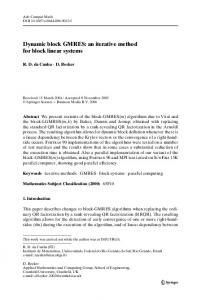
To examine the effectiveness of the block iterative method, let us consider a block of two node points as shown in Figure 1 and defined as

 4 − 1  U i, j   S1  =    − 1 4  U i +1, j   S 2 

(4)

where

S1 = U i , j −1 + U i, j +1 + U i −1, j , S2 = U i +1, j −1 + U i +1, j +1 + U i + 2, j . Determining the inverse matrix of the coefficient matrix in Eq. (4), the general scheme of the 2 Point-EG iterative method can be written as (Evans [2, 3]; Ibrahim [4])

 U i , j  1 4 1   S1   =    U i +1, j  15 1 4  S2 

(5)

The implementation of the 2 Point-EG iterative method as shown in Eq. (5) can be shown as

U i, j = U i +1, j

1 (4S1 + S 2 ) , 15 1 = (S1 + 4 S 2 ) . 15

(6)

2.5

∂ 2U ∂2x

+

∂ 2U ∂2 y

=0

(2)

By using the second-order central difference scheme, we can simplify the five point second-order standard finite difference approximation equations for problem (2) as generally stated in the in Eq. (3).

i-1,j

i,j+1

i+1,j+1

i,j

i+1,j

i,j-1

i+1,j-1

i+2,j

Figure 1: Illustration of a block of two node points to be considered for 2 Point-EG method.

3.0 SIMULATION In a static environment, the goal and the obstacles are fixed. Once the path has been generated, in can be reused as often as desired. The path generation proceeds very fast, since it only involves evaluation of the heat flux over a known temperature potential. Path planning in very simple mazelike environment is shown in Figure 2.

(b) (a) Figure 2: Illustration in (a) 3D View and (b) 2D view of paths generated from a numerical solution of Laplace’s equation.

Table 1: Number of iterations and maximum error for the three numerical techniques.

Number of iterations Maximum error

Jacobi

Gauss-Seidel

2 Point-EG

31,604

16,492

12,584

9.9977e-11

9.9933e-11

9.9954e-11

The maze shown in Figure 2 represents an area of approximately 100x100 units. The box denotes the goal point which was placed in the maze, and solid circle denotes starting point. Several dot circles represent obstacles were placed in the maze. Error tolerance is set at ε = 10−10 . The number of iterations required to solve this

maze is shown in Table 1, where 2 Point-EG proved to be faster compared to the other methods. The paths shown here were constructed by performing a steepest descent from start point to the goal, using only the grid points. Interpolation of the gradient would provide smoother paths.

3.0 CONCLUSION Harmonic functions offer a fast method of producing paths in a robot configuration space. Three numerical techniques were compared in this study for solving Laplace’s equation. In this experiment, it can be concluded from the results that the EG performs faster the standard numerical techniques. The 2 Point-EG iterative method is 31% faster than the standard Gauss-Seidel and more than 150% faster than the Jacobi. 4.0

REFERENCES

[1] Connolly, C. I., & Gruppen, R. 1993. On the applications of harmonic functions to robotics. Journal of Robotic Systems, 10(7): 931–946.

[2] Evans, D. J. 1985. Group Explicit Iterative methods for solving large linear systems. Int. J. Computer Maths., 17: 81-108. [3] Evans, D.J & Yousif, W. S. 1986. Explicit Group Iterative Methods for solving elliptic partial differential equations in 3-space dimensions. Int. J. Computer Maths., 18:323-340. [4] Ibrahim, A.. 1993. The Study of the Iterative Solution Of Boundary Value Problem by the Finite Difference Methods. PhD Thesis. Universiti Kebangsaan Malaysia. [5] Khatib, O. 1985. Real time obstacle avoidance for manipulators and mobile robots. IEEE Transactions on Robotics and Automation 1:500–505. [6] Koditschek, D. E. 1987. Exact robot navigation by means of potential functions: Some topological considerations. Proceedings of the IEEE International Conference on Robotics and Automation: 1-6. [7] Connolly, C. I., Burns, J. B., & Weiss, R. 1990. Path planning using Laplace’s equation. Proceedings of the IEEE International Conference on Robotics and Automation: 2102–2106. [8] Akishita, S., Kawamura, S., & Hayashi, K. 1990. Laplace potential for moving obstacle avoidance and approach of a mobile robot. Japan-USA Symposium on flexible automation, A Pacific rim conference: 139–142. [9] Sasaki, S. 1998. A Practical Computational Technique for Mobile Robot Navigation. Proceedings of the IEEE International Conference on Control Applications: 13231327.

[10] Sulaiman, J., Hasan, M.K. & Othman, M. 2007. Red-Black EDGSOR Iterative Method Using Triangle Element Approximation for 2D Poisson Equations. In. O. Gervasi & M. Gavrilova (Eds). Computational Science and Its Application 2007. Lecture Notes in Computer Science (LNCS 4707): 298-308. Berlin: Springer-Verlag. [11] Daily, R., & Bevly, D.M. 2008. Harmonic Potential Field Path Planning for High Speed Vehicles. In the proceeding of American Control Conference, Seattle, June 11-13, 46094614. [12] Willms, A.R. and Simon X.Y. 2008. IEEE Trans. on Systems, Man, and Cybernetics – Part B: Cybernetics, Vol. 38. No. 3, June 2008. Real-Time Robot Path Planning via a Distance-Propagating Dynamic System with Obstacle Clearance.

[13] Jan. G.E., Chang, K.Y., and Parberry I. 2008. Optimal Path Planning for Mobile Robot Navigation. IEEE/ASME Trans. on Mechatronics, Vol. 13, No. 4, Aug 2008, pages 451-460. [14] Bhattacharya, P. and Gavrilova, M.L. 2008. Roadmap-Based Path Planning - Using the Voronoi Diagram for a ClearanceBased Shortest Path. IEEE Robotics & Automation Magazine, Volume 15, Issue 2, June 2008. Page(s):58 – 66.