configuration space, in the presence of fixed obstacles. ... Keywords: Robot, path planning, combinatorial optimization, multi- .... a convention for transforming a configuration q â C into a canonical one giving .... of its center are given by ck.
Optimization Techniques for Robot Path Planning Preprint? Aleksandar Shurbevski, Noriaki Hirosue, and Hiroshi Nagamochi Department of Applied Mathematics and Physics, Kyoto University, Yoshida-Honmachi, Sakyo-ku, Kyoto 606-8105, Japan {shurbevski,n_hirosue,nag}@amp.i.kyoto-u.ac.jp
Abstract. We present a method for robot path planning in the robot’s configuration space, in the presence of fixed obstacles. Our method employs both combinatorial and gradient-based optimization techniques, but most distinguishably, it employs a Multi-sphere Scheme purposefully developed for two and three-dimensional packing problems. This is a singular feature which not only enables us to use a particularly high-grade implementation of a packing-problem solver, but can also be utilized as a model to reduce computational effort with other path-planning or obstacle avoidance methods. Keywords: Robot, path planning, combinatorial optimization, multisphere scheme, packing problems
1
Introduction
Robotics is already a well-established area vastly adopted in the domains of industry, entertainment, and steadily moving on to be incorporated in daily life. Yet still, there are many challenges left to be solved or improved upon. Among them is certainly the most fundamental robot motion planning, which becomes ever more challenging as the autonomy and our expectations of robots increase; “The minimum one would expect from an autonomous robot is the ability to plan its own motions” [1]. Motion planning in its essence is defined as the problem of finding a collisionfree continuous motion of one or more rigid objects from a given start to a known goal configuration. Commonly also referred to as the Piano Movers’ Problem [2], the basic problem investigates the movement of a single body, assumes complete and accurate knowledge of the environment, and neglects dynamic and kinematic issues, or the possibility of interaction and compliance of objects, however, many extensions have been built upon this simplified model. The one closest to this investigation is the Generalized Mover’s Problem [3], which deals with the motion ?
Full paper DOI:10.1007/978-3-319-01466-1_10, available online at http://link. springer.com/chapter/10.1007/978-3-319-01466-1_10
2
A. Shurbevski et al.
of an object comprised of multiple polyhedra, linked at various vertices (akin to a robotic arm with multiple joints). Furthermore, motion planning as conceived for the purpose of robotics has recently found its way into such diverse areas as video animation, or even biomolecular studies, where it has been used to study protein folding [4, 5]. For the reasons above, motion planning has gathered a lot of attention, and extensive research has been done. Notably, it has been proven to be computationally intractable [3, 6], with complexity increasing exponentially, not only with the degrees of freedom (DOF) of a robot, but also with the number of nonstatic obstacles [7]. Exact algorithms for motion planning do exist, however they adopt overly simplistic models which have little applicability in practice [8]. To alleviate the intrinsic computational complexity of robot path planning, several heuristic approaches have been developed, largely classified as Roadmap and Potential Field methods [1, 9, 10, 11]. It is notable that sampling based methods, such as the roadmap methods [12, 13] tend to incorporate a sort of potential field as well, and utilize the information which the intensity and gradients of this potential field can render with regard to the robot’s configuration space. A comparative overview of probabilistic roadmap planners can be found in [14]. Our approach falls under the umbrella of roadmap methods. In particular, it is aimed to extend ideas presented in [1, 15]. As a distinguishing feature, we use ideas purposefully developed for packing problems, such as the Multi-sphere Scheme [16], which is particularly useful in determining and penalizing collisions between objects [17], but also as a basis to implement object separation algorithms [18]. Moreover, using methods developed in two and three-dimensional packing solvers can greatly benefit our attempts to find collision-free configurations, with a very clear relation to interactions between physical objects.
2
Problem Description
Before proceeding we introduce formal description and notation used in the remainder of the paper. An object S is a closed continuous subspace in Rde , where R is the set of real numbers, and de ∈ {2, 3} is its dimension. A robot, R = {R1 , R2 , . . . , Rn }, is a collection of rigid objects connected at certain defined points, commonly called links and joints, respectively. To emphasize that individual objects in R are not entirely independent but have a high degree of mutual interaction, we also describe the robot as a multi-object system. The Euclidean space in which the robot operates is commonly called a workspace, denoted by W. (Note that the term workspace in some other publications is used to refer to the portion of Euclidean space reachable by the end-effector of a robotic arm [9].) We represent the workspace as Rde . A point r ∈ W is a de dimensional vector. We always denote a vector by a lower-case bold letter and assume it is of proper dimension. The workspace is populated by a collection O = {O1 , O2 , . . . , Om } of rigid and immovable objects, called obstacles. The obstacles can be of arbitrary shape,
Optimization Techniques for Robot Path Planning - Preprint
3
and we assume that we have complete and accurate knowledge of the obstacles’ geometry and spatial distribution.
θ2
θ2
qf
θ2
qc θ1
θ1 (a)
(b)
(c)
θ1
Fig. 1: A 2-DOF robot R in a workspace with obstacles along with its configuration space: (a) In a free configuration, R(q f ); (b) In a colliding configuration, R(q c ); (c) The configuration space C, represented as a torus, and non-free C-space shaded darker.
A key prerequisite of our problem is to be able to accurately determine the location of every point of the robot R in the workspace W. For that purpose, we use a configuration space, denoted by C [19]. The configuration space C is an abstract df -dimensional space (Fig. 1(c)), where df stands for the degrees of freedom of the robot. The role of configuration spaces and objects’ interactions in physical space are further discussed in Subsection 3.2. A point q ∈ C is called a configuration, and it uniquely defines the location of every point of R in W, that is, the robot’s position and orientation. However, the opposite is not true in general, for there may be (infinitely) many points in C corresponding to a single position and orientation of the robot. We have resolved this issue by adopting a convention for transforming a configuration q ∈ C into a canonical one giving the same position and orientation in the workspace. Therefore, it is justified to equate the terms “position and orientation” (in W-space) with “configuration” (in C-space). We write R(q) for the robot assuming configuration q ∈ C. The robot R has either natural or imposed restrictions on its range of motions, reflected as a restricted domain in C-space. In general, there are restrictions j j on each degree of freedom of the robot. Let D = {(rmin , rmax ) | j = 1, 2, . . . , df } j j be a set of ordered pairs, where (rmin , rmax ) gives respectively the minimum and maximum values for the j th degree of freedom. Thus, an ordered pair j j (rmin , rmax ) ∈ D defines the admissible range of values of q j , j = 1, 2, . . . , df , for which R(q) is still valid. We call the obstacles from W projected onto the configuration space, that is, areas B = {q ∈ C | ∃ Ok ∈ O s.t. R(q) ∩ Ok 6= ∅}, C-obstacles, and we call configurations q ∈ B collision configurations. Furthermore, there might be such configurations q ∈ C for which if the robot assumes the position and orientation R(q) in W-space, individual links Ri and Ry , i, y = 1, 2, . . . , n, i 6= y come into contact with each other at points other than the predefined joints, called selfj j collision configurations. Points q ∈ C, with rmin ≤ q j ≤ rmax , j = 1, 2, . . . , df , that are neither collision nor self-collision configurations are called free C-space,
4
A. Shurbevski et al.
and denoted by Cfree . For a configuration q ∈ C that is also in Cfree we say to be a free configuration (Fig. 1(a)), otherwise we say it is colliding (Fig. 1(b)). It is now possible to state more accurately the Motion Planning Problem: Instance: A robot R with df degrees of freedom and a set D of restrictions on the degrees of freedom, a set O of stationary and rigid obstacles with accurately determined geometry and locations in the workspace W. Query: Given an initial configuration q s ∈ C and an objective configuration q t ∈ C, both of which are in Cfree , find a continuous motion of R through the workspace W from R(q s ) to R(q t ) obeying DOF constraints, D, without any part of the robot, Ri , i = 1, 2, . . . , n coming into contact with any of the obstacles in O, nor with another part Ry , y = 1, 2, . . . , n, y 6= i of itself. From the perspective of C-space, the aim is to find a continuous curve (path) from q s to q t lying entirely in Cfree and not breaching any DOF constraint at any time. Such a path connecting q s to q t (∈ C) is said to be feasible. It is not always certain that a feasible path exists.
3
Solution Framework
As stated in the Introduction, the Robot Motion Planning problem has attracted a lot of interest since its inception, and the literature boasts an abundance of ideas and approaches. Even though the approach we present can clearly be identified as belonging to the class of Probabilistic Roadmap Methods [1, 9, 14, 15, 20], what primarily sets it apart from existing approaches, is that to the best of our knowledge, it is a first one to adopt methodologies specifically developed with packing problems in mind. We expect this to greatly aid the search for a feasible path, for both problems share some common features, namely, we need to efficiently tell if two objects (of arbitrary shape, position and orientation) in de -dimensional space overlap or not, even more, calculate the level of overlap, or penetration depth (to be more precisely defined in Subsection 3.3). Further still, once we have established that there does exist an overlap, we need to resolve it in an efficient manner, both with regards to computational effort, and fitness to contribute towards finding a feasible solution. The two main tools we have adopted are: The Multi-sphere Scheme [16], used to represent (approximate) an object in de -dimensional space by a set of de -dimensional spheres. This greatly facilitates the procedure for checking if two distinct objects intersect or not [17] and also calculating the penetration depth of this intersection. We shall use the abbreviation MSS for Multi-sphere Scheme. Nonlinear Programming Optimization Solver [18, 21], used in coupling with MSS to efficiently resolve intersections of two objects (of arbitrary complex shape) in W-space. In the remainder of this section, we will briefly overview the tools essential for tackling the problem.
Optimization Techniques for Robot Path Planning - Preprint
3.1
5
The Probabilistic Roadmap Method, PRM
Following is but a short review of certain notions from PRM (for Probabilistic Roadmap Method) [9, 14, 15] important to the presentation of our approach. It is not aimed at describing the method itself, but just as a glossary of terminology associated with it. The planning procedure with PRM consists of two phases: A learning phase, and a query phase. We carry out computationally and time demanding operations as a preprocessing in the learning phase, so that we will be able to almost instantaneously answer arbitrary queries. In the learning phase, we begin with a set O of rigid and immovable obstacles in W-space, as well as a description of a robot R together with the set D of DOFconstraints. The learning phase itself is a two-step process, having a construction step and an expansion step. In the construction step we perform random sampling of the df dimensional configuration space of the robot in an attempt to “learn” about the features of Cfree . Let V be a set of sampled points of Cfree . While sampling, we also try to connect pairs of sampled points. The choice of a candidate pair is done by a heuristic function estimating their distance in C-space. The procedure by which we try to make this connection is referred to as a local planner. We store the information of pairs connected by the local planer in a set E. Thus we have obtained a graph structure G = (V, E), the set V is the graph’s vertices, and E - the graph’s edges. In the following, we will refer to the graph G as a roadmap. The construction step terminates after a predefined time limit has been reached, or a certain population size of sample points in Cfree has been obtained. However, it is very likely that the resulting roadmap consists of several isolated components and does not accurately reflect the topology of C-space. The expansion step, which is the second step of the learning phase, aims to increase the connectivity of the roadmap. Regions where Cfree is connected while there is a gap between components in the roadmap are considered “difficult”. They might correspond to such regions in W-space as narrow passages or regions cluttered with obstacles. We aim to populate these regions of C-space with configuration samples so as to make a connection between different components of the roadmap. One of the features our approach boasts is that it sometimes relies on a sophisticated packing-problem solver to aid a local planer when trying to produce new candidate configurations. After the learning phase is done, we can use the obtained roadmap to perform multiple queries for a given robot and a set of obstacles. Queries (q s , q t ) are answered by trying to connect q s and q t to some vertices in V and then use a graph search algorithm to find a path which connects them in G. 3.2
Objects and their Interactions in Space
In this subsection we only touch upon notation essential for the exhibition of our proposed approach. We have followed standard geometric notions and their implementation as can be found in [1, 9, 19, 22].
6
A. Shurbevski et al.
Following the robot definition, we say that an object S is given in the workspace, W. A translation of an object in the workspace by a vector x ∈ W can be achieved by a Minkowski sum: S ⊕ x = {s + x | s ∈ S} .
(1)
We will be mainly interested in overlapping objects, as in Fig. 2(a). Given two overlapping objects, S and T , their penetration depth is judged according to: δ (S, T ) = min {kxk | S ∩ (T ⊕ x) = ∅, x ∈ W} .
(2)
The calculation of δ (S, T ) is a highly non-trivial task. There do exist clever methodologies proposed for determining if two polygons in the plane intersect or not, but in the interest of space we refrain from further discussion. The interested reader is referred to [18] and references therein. Working with movable objects in W has been simplified with the introduction of the configuration space, C. Let Λ(s, q) : W ×C → W be a motion function [18], taking as argument a point s ∈ W and a configuration q ∈ C, and moves the point s by q-variables. The choice of a motion function for a given robot may not be unique, but we adopt conventions by which C is always a differentiable manifold [9]. Thus, an object S in configuration q is given as: [ S(q) = Λ(s, q). (3) s∈S
Configurations of robots as articulated multi-object systems are a composition of configurations for each individual object, and certain relations between them exist, depending on the robot’s representation as a serial or a parallel mechanism. 3.3
The Multi-sphere Scheme, MSS
The Multi-sphere Scheme [16] has been devised as a framework aimed to simplify certain geometrical issues commonly arising in packing and cutting stock problems [18]. It has gone beyond a mere approximation of geometrical objects for the purpose of fast collision detection [23]. In addition to the original application [18], MSS has continued to evolve [24, 25], and has since been applied in fields such as layout planning and optimization [26, 27], and the present, robot motion planning [28, 29]. Without further ado, we state that we have a means of approximating any solid object, say Ok , in Rde by a set {O1k , O2k , . . . , Onk k } of nk de -dimensional spheres. Details on how to obtain such an approximation from other types of object representations can be found in [25]. In the context of MSS, we shall use Ok to denote both an object and the set of spheres used to approximate it. Now the object Ok can be though of as a multi-object system consisting of nk spheres, where the sphere Oik has radius rik , and the coordinates of its center are given by cki ∈ Rde . The motion of the object Ok retains the form of Eq. (3), only the union is over all spheres in Ok , a finite number. As already mentioned, MSS greatly facilitates the procedures we need to recognize if two distinct objects ever come into contact with little computational effort. Further still, we would like to be able to also quickly compute the amount
Optimization Techniques for Robot Path Planning - Preprint
7
(a) (b) (c) (d) Fig. 2: Objects in de = 2-dimensions: (a) Two overlapping objects; (b) A coarse MSS approximation; (c) A finer MSS approximation; (d) MSS approximation with spheres of variable radii.
of overlap between two colliding objects. Let Ok and Ol be two objects in Rde , each approximated by a set of spheres. For brevity, we ommit stating their configurations explicitly. For two spheres Oik ∈ Ok and Ojl ∈ Ol , the penetration depth function from Eq. (2) can be simplified to:
� � (4) δ Oik , Ojl = max rik + rjl − cki − clj , 0 . In addition to the penetration depth, for two spheres of different objects, Oik ∈ Ok and Ojl ∈ Ol , we introduce the penetration penalty function: � ��2 pen fijkl Oik , Ojl = δ Oik , Ojl (5) and the overall penetration penalty function for two objects, Ok and Ol , becomes: fpen (Ok , Ol ) =
nk X nl X
pen fijkl Oik , Ojl
�
(6)
i=1 j=1
Since the robot R was initially given as a multi-object system (Section 2), we write Ri (q) for the link Ri ∈ R as it is when the configuration of the robot is given by q, for notational convenience. As the robot R is assumed to be the only movable object in a given instance of R, O in W, it is the only one for which explicitly defining a configuration makes sense, therefore the notation Oj (q), j = 1, 2, . . . , m is omitted and obstacles are simply referenced as Oj ∈ O. We introduce a penalty function Fpen (q), q ∈ C depicting intersection penalties in the entire scene (R(q), O): Fpen (q) =
m n X X
fpen (Ri (q), Oj ) +
i=1 j=1
3.4
X
fpen (Rk (q), Rl (q)) .
(7)
1≤k