830
IEEE TRANSACTIONS ON INSTRUMENTATION AND MEASUREMENT, VOL. 53, NO. 3, JUNE 2004
Block-Oriented Instrument Software Design Yves Rolain, Senior Member, IEEE, and Wendy Van Moer, Member, IEEE
Abstract—A new method for writing instrumentation software is proposed. It is based on the abstract description of the instrument operation and combines the advantages of a reconfigurable instrument and interchangeability of the instrumentation modules. The proposed test case is the implementation of a microwave network analyzer for nonlinear systems based on VISA and plug and play instrument drivers. Index Terms—Automated measurements, instrumentation software, programming, software engineering.
I. INTRODUCTION
T
HE CURRENT trend in instrumentation to move away from “raw” instruments, that measure one fundamental quantity, toward “parameter extractor setups,” that measure almost any derived quantity, has moved the instrumentation focus away from the custom hardware. “Modern” instruments—or instrumentation setups—are likely to be built up around generic hardware and custom software. The advantage of this evolution is the possibility to “measure” about anything. The disadvantage is that the amount of software required to operate such a device or setup is very high and so is its complexity. An acceptable development time for a reasonably low number of software bugs can, therefore, only be obtained if the software is maximally reused from earlier developments. Several attempts have been made in the past to realize this. Most attempts used a two-step approach. In a first step, the transport interface between computer and instrument is abstracted. Second, the instrumentation command is abstracted to empower the interchangeability of similar pieces of instrumentation. The first step in this approach has always been quite successful. To our knowledge, the first transport abstraction stems from the IEEE-488 interface. Afterward, SICL and VISA were developed to support multiple transport buses (IEEE-488, RS-232 and, later, Ethernet and IEEE-1394). These methods use a file as the conceptual model for an instrument. The commands sent to the “files” are independent of the transmission medium, medium dependency is localized only in the initialization call. Most interfaces that can be used for instrumentation control are, hence, supported by these frameworks. For the second step, the situation always has been much less obvious. A first significant contribution has been introduced in the IEEE codes and formats specifications. The main idea here Manuscript received February 19, 2003; revised March 4, 2004. This work was supported in part by the Fund for Scientific Research (FWO-Vlaanderen), the Flemish Government (GOA-IMMI), and the Belgian Government (Interuniversity Poles of Attraction IUAP V/22). The authors are with Electrical Measurement Department (ELEC), Vrije Universiteit Brussels, B-1050 Brussel, Belgium (e-mail:
[email protected]). Digital Object Identifier 10.1109/TIM.2004.827310
was that programming instrumentation is far easier if the data streams that circulate between “controller” and “instrument” have a standardized format. Besides a standardization of the text formats, one of the important contributions here is the standardization of the binary data transfers. This led to the IEEE floating point formats, which are in general use nowadays for the transfer of floating point data between computer platforms. However, the formatting specification has only been loosely adopted by the instrumentation manufacturers. Despite its significance, this approach does not completely solve the problem of instrument interchangeability; to be able to replace similar instruments in the code without reprogramming, there is also a need for a syntactical and semantical standardization of the commands that are to be sent to the devices. A first vein of solutions used an old programmers trick to solve the problem: “define a language for each problem you encounter.” Even if such an approach solved the problem in a theoretical setting, none of the methods based on this principle really survived practical use. In the definition phase, the languages are defined to be nonoverlapping and follow a clear cut set of rules. This results in a limited command set that is easy to learn, since it is supported by clear syntactical and semantical rules. In a second phase, instrument designers start to implement the language on their new designs. Due to both a poor understanding of the rules used to define the language and the will to bind users to a particular brand of instruments, the command set starts to grow in an exponential way. Overlapping commands are then defined, and finally a separate command set is almost added to the standard for each new instrument. This is exactly what happened to the standard commands for programmable instrumentation (SCPI) language which defines a standard set of commands to control programmable test and measurement devices in instrumentation systems. A second vein of solutions uses the concept of a custom code library to control each device separately. Originally, the idea was to define a majority of standard calls that should have been sufficient to operate the device in such a library. Device-specific options were then allowed to be defined in additional calls to increase device performance. Gradually, the idea has been eroded as the number of standard commands decreased and the number of custom calls increased. Finally, the leftovers consist of an empty bag of standard commands that do almost nothing anymore and are only added to the driver to be able to claim standard compliance. This has been the scenario for the plug and play (PnP) driver standard. Some one-step methods have also been used with variable success. Graphical fourth generation programming languages, such as those used in LabVIEW and VEE, are a blessing for simple setups, with a limited number of instrument interactions. They require a separate driver for each instrument an, hence,
0018-9456/04$20.00 © 2004 IEEE
Authorized licensed use limited to: Rik Pintelon. Downloaded on December 2, 2008 at 08:41 from IEEE Xplore. Restrictions apply.
ROLAIN AND VAN MOER: BLOCK-ORIENTED INSTRUMENT SOFTWARE DESIGN
Fig. 1.
831
Block schematic of the two-port network analyzer.
lack the instrument interchangeability feature. Therefore, they do not solve the problem that is considered in this paper. Taking one step back, it is striking that almost every proposed method had the capability to solve the interchangeability problem. The failures stem from the fact that the manufacturers are required to implement the standard while, on the other hand, their main concern lies in keeping the end users away from the competition. Only the end users have something to gain in instrument interchangeability, and they have no contribution in the methods defined so far. In this paper, a different approach is taken where the end user plays the key role. An abstract model to programming instrumentation setups is proposed, which is easy to understand for an instrumentation practitioner and general enough to be used for complex setups. The feasibility of the proposed method is shown in several examples. II. CONCEPTUAL IDEA BEHIND THE PROPOSED METHOD In this paper, an approach is proposed that is user-centric rather than instrument-centric. The main hypothesis, therefore, is that the end user does know what is to be measured and how it has to be measured conceptually. The solution will be composed at an abstract level starting from the user requirements. To avoid a steep learning curve and maintain the user in a familiar environment, this definition phase is performed using a block schematic diagram. This representation is easy to read and understand to an instrumentation user, but still contains all the important information that leads to a successful implementation. The block schematic diagram is a graphical functional representation of the data transformations performed inside an instrument. It consists of blocks which represent elementary actions, and lines, that stand for analog or digital signals. The blocks can be grouped into different classes, as follows. 1) Signal generation nodes: Act as a source for some signal. This includes RF signal sources, dc sources, function generators, and arbitrary waveform generators, but also clock generators and trigger sources. 2) Signal acquisition nodes: Transform the signal or its replica to a measured quantity. Analog-to-digital convertors; power meters and volt and ampere meters belong to this class.
3) Signal processing nodes: Modify some properties of a signal. This class contains frequency convertors, filters, amplifiers, switches, and couplers. 4) Device under test (DUT): The DUT is the essential part of the setup, which is to be characterized. Its inclusion in the schematic allows the connections between the instrument and the device. The signals can be further separated into three different classes, as follows. 1) The data signals are the information carriers. They convey replicas of the observed quantities. 2) The clock signals are the timing carriers. They synchronize time in between the different nodes. 3) The trigger signals are event carriers. They synchronize the actions performed by the instrument. Also, it will then be assumed that the knowledge contained in the block schematic diagram is sufficient to operate an abstract device that mimics the behavior of the real-world device perfectly. This hypothesis is introduced as such because it is not straightforward to prove that the translation from block schematic to a real instrument is always possible. To prove that this hypothesis is not very restrictive, several instrumentation setups were developed using the proposed framework, as will be shown later in the paper. The usefulness of the description is illustrated by the example of the realization of an RF network analyzer shown in Fig. 1. Depending on the bandwidth of the used acquisition channels (ACQ) and the settings of the sample clocks, this network analyzer is capable of measuring the linear response or the nonlinear response of the DUT. The members of the signal generation group are labeled using a circular shape. Two types of devices are present: the RF generator, which is essentially a sinewave generator at high frequencies, and the clock generator, which provides a common time reference for all blocks. The acquisition group is represented by ACQ blocks only. Note that these blocks have two inputs: the signal to be measured and the sampling clock. The signal processing group is the most populated in this setup. Each signal measurement path contains a coupler to separate waves and a sampling downconvertor to obtain a low-fre-
Authorized licensed use limited to: Rik Pintelon. Downloaded on December 2, 2008 at 08:41 from IEEE Xplore. Restrictions apply.
832
IEEE TRANSACTIONS ON INSTRUMENTATION AND MEASUREMENT, VOL. 53, NO. 3, JUNE 2004
quency replica of high frequency waves. Sampling rate convertors (also called fractional N counters) are used to change the frequency of the clock signals without losing the phase coherence with the input signal. The DUT is included in the setup, as it is an essential part in the measurement operation. The signals that are present also belong to different groups, as follows. 1) The data signals, labeled using open arrows , describe both the main signal path flowing from the RF generators to the DUT and the measurement signal paths from the couplers to the ADC. These are the primary paths to exchange information between instrument and DUT. , 2) The clock signals, labeled using filled black arrows show that the generators and acquisition modules remain phase coherent and that the acquisition modules are operated synchronously: the signals to be measured are all sampled at the same instant in time. 3) The trigger signals, labeled using closed arrows, show that the TRIG source starts the four acquisition signals simultaneously, resulting in a measurement acquisition window that is synchronized on the four channels. III. STRUCTURE INSENSITIVE INSTRUMENTATION METHODS Instrument interchangeability is now included by design in the proposed method: any instrument that provides the required functionality that is described by the abstract blocks can be plugged into the setup and can be used to implement the abstract node. Can one now optimize the reusability of the instrumentation code based on the same approach? In the ideal world, a measurement procedure should be independent of the actual structure of the instrument itself. As long as the elements that are required to execute this measurement procedure are present in the actual setup, the software should not be reprogrammed, but it should automatically adapt itself to the new instrument structure. This is, theoretically speaking, always possible when the required functionality is present in the actual instrument. To make this point more clear, consider the following example. The network analyzer used in Fig. 1 can be extended to excite the DUT with complex modulated signals instead of simple sinewaves. In that case, the simple generator setup of port 1 (see left-hand side scheme in Fig. 2) is replaced with a modulated setup as shown in the right-hand side of Fig. 2. Consider, now, that the network analyzer setup is to be calibrated; then, the truly reusable code should not be changed in any way to perform the calibration for either one of the setups, since the more complex setup can be made to behave as the more simple one if no modulation is enabled. To achieve this goal, it is mandatory that the user code does not rely on a known instrument structure. An additional level of abstraction is, therefore, required to hide the specific topology of the setup. In a measurement context, statements such as “the incident power from port 1,” or “the frequency applied at port 1” are quite common. This indicates that in the user’s mind, the natural interface between DUT and instrument is a measurement port. Measurement ports will, therefore, also be used as
Fig. 2. Generator setup for a modulated experiment.
the additional abstraction level during the development of the instrumentation code. The instrument block schematic diagram is extended to incorporate these ports, as shown in Fig. 3. Note that these ports have different types of terminals, each with their specific semantic signification. The DUT terminal links the measurement port with the world outside the instrument. The ports labeled “a” and “b,” in this case, are the port variable terminals. They are chosen to fully describe the port operation of the device (in the system theoretic sense). The terminal labeled “g” is the generator terminal that is used by the instrument to excite the DUT. The user and instrument interact only through these ports. The general structure of the commands will, therefore, contain the command descriptor, the terminal descriptor of the port terminal to which the command is to be sent, and the command parameters. This clearly enables a code reusability concept that goes further than just the swapping of almost identical devices, and opens the way to more reliable and cheaper-to-develop instruments, as shown in the following example. The power of the structure-independent abstraction is then illustrated on the example of a network analyzer measurement at a single frequency. The whole measurement setup boils down to a few lines of code. In the example above, this results in a pseudocode statement, such as the following: GHz dBm
(1) (2) (3) (4) (5) (6) (7) (8)
The tasks accomplished by these commands will be described in a little more detail. For (1), a block with the functionality of an RF generator is sought through the generator connector of port 1. The generator is directly connected to the port and the block is retrieved. The “SetFrequency” command is then sent to this block, and can be executed as setting the frequency in one of the operations that are supported by the RFGen generic device. The same execution scheme is then repeated for the power setting of the same generator. The third line deserves some more attention. The star acts as a wildcard that will match any character and will propagate the specified command to all the modules of the appropriate type that are connected to one of the ports of the setup. Blocks of type ACQ are, therefore, searched along
Authorized licensed use limited to: Rik Pintelon. Downloaded on December 2, 2008 at 08:41 from IEEE Xplore. Restrictions apply.
ROLAIN AND VAN MOER: BLOCK-ORIENTED INSTRUMENT SOFTWARE DESIGN
Fig. 3.
833
Measurement port as an abstraction between use and instrument.
all the signal paths of both ports. The propagation starting from terminal “a1” happens as follows. Terminal “a1” is connected to a downconvertor (DC) block. Since this is not an ACQ block, the propagation is continued through the signal input connection of the DC. The next block is an ACQ and, hence, a reference to this block is returned to the initiating call. A similar execution on the other port terminals yields the four ACQ blocks in the setup. The command is then executed in turn using this list of references to instruments. In (4), the trigger generator connected to “a1” is located first and a synchronous acquisition on the four ACQ modules is started next. The last four lines are used to retrieve the measured data from the four ACQs. After these seven pseudocode lines, all the measurements for a full analysis at one frequency are taken. Note that the actual structure of the instrumentation network is not used. Exactly the same code can be used to perform the measurement on a totally different set of hardware, as long as it has the capability of doing such a network analysis data capture. Note that during this explanation, it was always assumed that the block that is to receive the command can be uniquely identified given a port terminal and a block functionality. Unfortunately, this is not always true, in general. Under some circumstances, a search for a specified block functionality may return more than 1 block. To identify the block that is to be used to execute the command, there is a need to allow further discrimination between the returned nodes. Furthermore, the nodes can also be labeled using a node name. To avoid the burden of having to specify the node names in all the calls, the names will only be used in the special cases where the ambiguity exists. An example of how to handle these quite rare cases is given in the third example in Section XI.
IV. NETWORK REPRESENTATION OF INSTRUMENT SETUPS At this moment, a conceptual model for the instrumentation setup has been defined. What remains now is to translate this into a software framework that is sufficiently flexible for the high-level operations and also easy to reconfigure. The choice of a network of object instances is straightforward, as the diagram is itself a network of nodes. The basic properties to be allocated to a generic node are also quite easy to derive. A node can be connected to other nodes
Fig. 4. Definition of the generic module and its signal interactions.
Fig. 5.
Definition of the generic port module and its signal interactions.
by means of a clock signal, a data signal, or a trigger signal. Each node can be connected to more than one node on each used connector. The generic node in a setup, therefore, requires three types of connectors: clock, signal, and trigger connectors. Since a node can either sink or source such a signal, the generic node has six connections, as shown in Fig. 4. Each block in a graph is translated into a node that inherits this structure and is further specialized in order to implement the requested functionality, as seen later. In addition, the node also requires a link to the instrument hardware that is to be used. To minimize the configuration effort, the user specifies only an address reference to the instrument under PnP compliant format. The required information about the model and/or manufacturer of this device is retrieved automatically by the framework. This both reduces the burden on the user and minimizes the probability for an error to be introduced in the setup. Since a command is always launched from a port, it is clear that the port will need to have a special structure. There, the signal path is further specialized into two connectors to measure the port quantities. The regular signal path is then connected to the DUT on one side and on the generator on the other one, as shown in Fig. 5. To show that this way of abstraction leads to a useable result, the example block schematic diagram of Fig. 1 is then translated into the network of nodes shown in Fig. 6. Note that considering the complexity of the instrument that is modeled, the model is still quite easy to understand for an instrumentation practitioner.
Authorized licensed use limited to: Rik Pintelon. Downloaded on December 2, 2008 at 08:41 from IEEE Xplore. Restrictions apply.
834
Fig. 6.
IEEE TRANSACTIONS ON INSTRUMENTATION AND MEASUREMENT, VOL. 53, NO. 3, JUNE 2004
!: signal, 0
Node network associated with the earlier example (
0
: clock, and .: a trigger connection.
V. DEFINITION OF THE GENERIC NODES The definition of the generic nodes to be included in the framework is one of the most delicate points in the definition of the framework. If the set of generic nodes is not rich enough to tackle a general application and the inclusion of user-defined nodes is to be added to ensure the wide applicability of the method, the risk is that the number of nodes will be increased beyond a reasonable limit. To avoid this, one has to meet contradictory requirements: the set of generic nodes has to be wide enough to describe a general instrumentation setup while the complexity of the whole network has to be low enough to allow an end user to understand the operation of the instrument. In any case, the situation is better for the end user, who can now partition an existing instrumentation box into a set of nodes. If there is no node representation available for an instrument, the user can take advantage of any existing driver to glue one together. One box can also be used to implement several different nodes. This can, in some cases, even result in overlap of functionality. Again, since the user has the freedom to adapt and tailor the node definition of an instrument box to his own needs, this does not pose any problem. A carefully tailored set of nodes is defined below. The generic node set is separated into five classes of nodes: signal generation nodes, signal acquisition nodes, signal processing nodes, clock nodes, and trigger nodes. To reduce the amount of instrument state information that the user has to maintain in software to the extreme minimum, each setting of each module can be set and retrieved from the instrument. Note that the retrieved value is always the actual
hardware value, and that it, hence, is rounded with the precision of the hardware setting. A. Signal Generation Nodes The signal generation nodes are grouped into two application-oriented classes: IF generators and RF generators, whose naming background stems from the original RF background of the framework. The RF class contains two CW (sinewave) sources: a fixed frequency source and a swept source. For these sources, the frequency (span) and the power of the tone can be set. The IF class is further subdivided, depending on the waveshape of the generated wave. An overview of the supplied functionality can be seen at the bottom of the page. A compromise had to be made between readability and normalization. The arbitrary waveform generator has no frequency setting because it uses an externally-supplied clock. The RMS amplitude of the signals is used for any generator excepted for the AWG, where the peak value is provided. B. Signal Acquisition Nodes Signal acquisition nodes contain all the nodes that convert a physical signal into a measured quantity. The most common acquisition module is certainly an ADC module. This module is labeled “ACQ” to show its common applicability. To reduce the number of nodes that are required to describe an A/D conversion, the functionality of the “ACQ” module has been extended. Besides the expected function “setBlockLength” to determine the number of samples and “setDelay” to handle the pre- or post-triggering, basic signal processing capability
Authorized licensed use limited to: Rik Pintelon. Downloaded on December 2, 2008 at 08:41 from IEEE Xplore. Restrictions apply.
ROLAIN AND VAN MOER: BLOCK-ORIENTED INSTRUMENT SOFTWARE DESIGN
has also been added: “setOffset” and “SetRange” determine the voltage window that is available for discretization. An autorange option is supplied to minimize the burden on the user. Finally, the “setCoupling” command allows for dc- or ac-coupled measurements. To allow for easy single triggering of a measurement setup, a “measure” call is used to start the acquisition of a data block. Besides this generic ACQ functionality, specialized modules were introduced to take care of basic RMS or dc current and voltage measurements. This leads to the introduction of the voltmeter, amperemeter, and wattmeter nodes. These nodes are assumed to take only one reading at a time. C. Signal Processing Nodes Up until now, the signal processing nodes were limited to analog nodes. However, this is not a limitation of the method, but rather the absence of the need for digital processing nodes. The analog processing nodes can be subdivided into signal conditioning nodes, such as filters, attenuators, amplifiers, variable impedances, and switches on one hand and signal modulation nodes on the other hand. For all these nodes, the bandwidth of the device is accessible through the calls. Of course, for all the fixed bandwidth devices, this is a read-only variable. Amplifiers and attenuators are used to set the correct signal level. The realized gain/attenuation is, therefore, the only additional programmable parameter. The variable impedance tuner node is used to realize a userspecified impedance at a certain frequency. The programmable parameters here are the frequency and the value of the complex impedance. Switches are used as a special signal conditioning node, as the information required to determine their state depends on the position of another node in the model network. The modulation devices include diverse nodes. The source modulators are used to construct spectrally rich excitation signals, such as multitones or noise. Depending on the actual shape of the output, phase modulators, amplitude modulators, frequency modulators, and IQ or orthogonal modulators are considered. The only parameter that is provided for these nodes is an activation switch. D. Clock Nodes Clocks are separated into oscillator and frequency dividing modules. Oscillator modules are assumed to be free running and, hence, are not phase coherent to one another. They are used for the time references that are used in the setup. In phase coherent setups, there is normally only one independent clock. For an independent clock, only the frequency of the clock can be set. All the other clocks are frequency dividers, multipliers, fractional N synthesizers, or clock interface modules. These nodes change the frequency or the physical carrier of the clock signal. An example of such a module is the sampling clock generator used in an ADC. For divider modules, the clock cannot be set; the multiplication and/or division factors of the clock are given instead. The interfacing behavior of the module is determined through its connections: if a clock module is connected to an external input clock signal and is used to clock a VXI bus module, it will attempt to connect the physical clock module accordingly.
835
E. Trigger Nodes Trigger nodes behave essentially like clock modules. Most trigger modules have an input and an output connection. The input then represents a physical signal that starts a certain card operation while the output tends to be a logical signal that will actually start a module task. For software triggers such as a “single” trigger function, the input signal is a software command. VI. BREAKING THE CURSE OF COMPLEXITY The complexity of the full block schematic diagram will be broken using meta-nodes, i.e., nodes that contain themselves a block schematic diagram of a whole setup. This allows complex instrumentation setups where the major part of the complexity is hidden from the end user. Currently, this approach has been successfully used to hide the complexity of the nonlinear network analyzer shown in the above examples. VII. ADVANTAGES OF A MODEL: SYNTHETIC DATA SOURCES One of the most frustrating feelings for an experimenter is to have gathered measurement data for a complex setup and then come to the conclusion that the experiment is to be done over again because some instrument settings are missing. Often, this results in experiments having to be done over again to get the infamous setting that was not written down earlier on. An ideal instrument would of course take care of this problem, as it would save all settings in such a way that a user can easily get them back out of the measurement data. On the other hand, the comparison of device specifications often requires several different devices to be measured under experimental conditions that are perfectly matched. From personal experience, we know that this often requires remeasurement of all the devices to make sure that “nothing has been forgotten.” Again, the ideal instrument needs a replay button that allows even the most complex measurement sequences to be repeated perfectly. The proposed framework allows a solution for both issues at a zero additional effort. Remember that the instrument is represented by the node network in the computer. Looking back at the programmable variables for all the network nodes as defined earlier, it is clear that the current state of the instrument is completely determined by the value of the programmable parameters. Put in another way, the current measurement can be repeated at any time if all the nodes of the instrument network are reloaded with their actual values. Given the network of nodes, it is also very easy to gather all these variables and to label them automatically. Putting all these names together and using them as the names of the columns of a database table, the instrument setup can now be represented by one row in this table. The table can be generated automatically by the measurement framework, as all the nodes are known to this piece of software. Since the interaction between user and network is restricted to happen through the ports of the instrument, it is also very easy to decide when a new measurement is started. When the
Authorized licensed use limited to: Rik Pintelon. Downloaded on December 2, 2008 at 08:41 from IEEE Xplore. Restrictions apply.
836
IEEE TRANSACTIONS ON INSTRUMENTATION AND MEASUREMENT, VOL. 53, NO. 3, JUNE 2004
Fig. 7. Measurement setup for the time-domain network analyzer.
instrument state is saved any time a new measurement occurs, the whole measurement session gets saved. Besides the state, the measurements themselves can also be saved automatically, as, again, the system can determine what measurement data can be saved and generate database tables to save this data. The data that is then retrieved by the user can be intercepted by the framework and saved automatically. The user can also choose to interact with this process, deciding, for example, to save processed data instead of raw data. The framework provides the calls to automatically link the derived data to the actual instrument status. One nice by-product of this database function is that it is perfectly possible to start a long measurement overnight, and then use exactly the same code to “measure” fictively in the morning, starting from the database that was constructed during the physical measurement to obtain the data a posteriori without having to perform a single change in the instrumentation code. VIII. PUTTING THE MODEL TO WORK A. Linking Real Instruments to Abstract Nodes To start the operation of the instrument, the instrument type and/or manufacturer are retrieved for all the nodes that are used in the network. This is required to translate the abstract commands issued by the instrument model to a specific set of instructions that the physical device understands and that perform the requested action. Since, in the current framework, the determination of the link between abstract and concrete nodes is postponed until runtime and is requested to happen without user interaction to minimize the load on the user, it is assumed that all the instruments used can identify themselves in some way. B. Initialization and Default Values Even if the importance of a good definition of an instrument model can hardly be overestimated, it is only one step in the implementation of a working instrumentation framework. The next step requires that this abstracted data structure is turned into an instrument setup that is properly configured and ready to perform the actual measurements. Since, in this paper, the ease of use for the instrumentation user is the major concern, the number of parameters that have to be configured by the user will be reduced to the strict minimum.
A crucial issue within this respect is the initialization of the different parts of the network. To avoid that the initialization of one module destroys the state of the other ones, the order in which the initialization is done is to be carefully engineered. The problem lies mainly in the clock and the trigger setup of the instrument. For the clock nodes, it is mandatory that the oscillator nodes are initialized first. If the oscillators of the setup fail to be initialized first, some devices can end up having no clock at all any longer. This can result in a dead lock situation, where the hardware can only be brought back to life through a power cycling or cold reset. In a second step, the setup is searched for ACQ nodes that operate as a phase coherent group, meaning that the cards are to be synchronized in such a way that the sampling on all the channels occurs simultaneously, even for cards with undersampling convertors. In such a group, one card operates as a master that generates the timing for the other ones that appear to be slaves, steered by the master. Automatic detection of master and slave modules is performed. The master is recognized since it has a clock input that comes from an independent source, and outputs it clock to the other members of the group. This results in a fully-automatic configuration of the group. In a third step, all the remaining clock nodes are initialized, starting from the ones that are the closest to the oscillator and ending with the ones that are most distant. To make things more clear, consider the initialization of the clock circuitry for the analyzer of the previous example. The only clock node that is an oscillator node is CLK1, since this node has no clock input. All the other clock nodes, therefore, are clock dividers/multipliers. CLK1 will, therefore, be initialized first and loaded with the appropriate initial frequency value. Both CLK2 and CLK3 are directly connected to CLK1, and, therefore, the order in which they are initialized is not critical. They will then be loaded with an appropriate initial division factor. An acquisition group, i.e., a group of ACQ that samples simultaneously, is detected in the node network. ACQ1 sources its clock from a different clock module than the three other ACQ modules. The last ones all get their clock from the same module, ACQ1. Therefore, ACQ1 is the master in the group and needs to be initialized before the slave modules. The order in which ACQ2, ACQ3, and ACQ4 are initialized is no longer critical.
Authorized licensed use limited to: Rik Pintelon. Downloaded on December 2, 2008 at 08:41 from IEEE Xplore. Restrictions apply.
ROLAIN AND VAN MOER: BLOCK-ORIENTED INSTRUMENT SOFTWARE DESIGN
Fig. 8.
837
Measurement setup for the spectrum analyzer.
For the trigger setup, a similar operation is to be performed. The order in which the different modules are initialized is the same as for the clock modules Finally, default values are loaded into the remaining nodes of the network. These values can be chosen by the designer of the instrument to avoid requiring users to configure a long list of parameters before to start measurements. IX. CONCRETE NODES: THE DRIVER LAYER The main issue for the driver layer is to standardize as much as possible the software drivers. The VISA standard [1] is used at any time for the transport layer abstraction. The VISA standard allows identical calls for IEEE-488, VXI, ethernet, or even serial programmable instruments. For register-based devices, the PnP standard for functional drivers has been used. Unfortunately, not all the cards that are used in the setup have available PnP drivers. The missing drivers have been written. In addition, the drivers that are available were often of poor quality and had to be debugged before they could be used. The implementation problem already starts with the device identification. If all the devices were to obey standard protocols such as IEEE-488.2 or VXI-PnP, the “ idn?” call would be sufficient to obtain the identification. However, the fact that many IEEE-488 devices do not support these standard calls, and that the IEEE-488 bus is an asynchronous bus lead to a quite complex custom procedure to identify all the devices hooked up to the instrumentation. Up to now, all the devices that were used could identify themselves in some way, but the number of different formats or commands almost equals the number of devices, especially for the elder IEEE-488 devices. The advantage of the framework within this respect is that, if a device requests such a “special treatment” for identification, this can easily be added by the user or the developer of the new setup. The different possible commands are then issued to each device in the order of probability of appearance and error handling is used to determine if the calls were successful. X. PRACTICAL MATLAB IMPLEMENTATION The VISA driver calls are glued inside Matlab 6 as Matlab extension (mex) files. Matlab calls are identical to the VISA calls to minimize the required documentation effort. The glue code fully supports the VISA attributes and pre-defined arguments. They can be passed as strings to the mex files. The glue code parses the Matlab arguments and performs the type conversions between Matlab and VISA types. The glue code has been developed in C++ using Microsoft Visual Studio.
The home-made PnP drivers for the cards were also developed in C++. The glue code to make these calls available in Matlab supports one generic call for each card type. This call is named according to the card type. The PnP function name is passed as the first argument to the generic call. The input arguments of the call are passed in the right-hand side of the Matlab expression, while the pointer references returned by the PnP call are passed in the leftt-hand side of the call. Since the order of the input and output parameters is respected, the original documentation of the PnP calls can also be recycled. The only disadvantage of the current implementation is that the introduction of a new VXI card requires the creation of a new glue library (see also [4]). However, the extensive use of utility libraries to perform the routine tasks limits the effort of the development to the strict minimum. XI. EXAMPLE IMPLEMENTATIONS The first example implements a full microwave nonlinear network analyzer based on the HP-85 120A-K60 prototype hardware. The computer platform is Pentium III Compaq Deskpro running Windows 2000. The VXI card cage is connected through the MXI slot zero controller and a National Instruments PCI-MXI 2000 card. The GPIB instruments are connected on a GPIB-PCI controller also from National Instruments. All the instrumentation interfaces are driven by the National Instruments’ VISA driver. The setup has been used in several different configurations, ranging from a CW excited setup to a multicarrier wideband modulated setup and even a broadband excitation setup (up to 2-GHz bandwidth). All the versions of the instrument were using the same code to perform the measurements. The calibration code used in all those experiments was exactly the same code also. Measurements performed with this setup are referenced in [6]–[8]. Next, a time-domain network analyzer was realized using an HP54121 TDR scope. The node network for this setup is shown in Fig. 7. The code to perform the measurements is the same as the one used in the first example. Even if a single box physical instrument was used in this case, a node network could still easily be derived. The advantage is that the device is then controlled using exactly identical commands as the ones used in the first example. Measurements performed using this setup are described in [5]. To show a different type of functionality, the setup used to control the spectrum analyzer in noise figure measurements of [9] is considered. The block schematic diagram for that setup is shown in Fig. 8. Note that setting the gain of an amplifier connected to port 1 now contains the kind of ambiguity that was predicted earlier. To
Authorized licensed use limited to: Rik Pintelon. Downloaded on December 2, 2008 at 08:41 from IEEE Xplore. Restrictions apply.
838
IEEE TRANSACTIONS ON INSTRUMENTATION AND MEASUREMENT, VOL. 53, NO. 3, JUNE 2004
address the requested amplifier through a connection via port 1, the system requires more than the type of the block, which is the reason why a block can also be named, using a name that refers to the functionality of the node. The combination node type + node name then uniquely identifies the block to be used. Finally, the code was also used to perform eight channel mechanical transfer function matrix measurements on a brake system. Again, the command set was identical. This has reduced the threshold for the use of complex VXI instrumentation setups significantly. XII. CONCLUSION A framework for the development for inter-operable, reconfigurable, and reusable instrumentation is proposed. The approach allows different instruments with similar capability to be exchanged without changing the code. The setup also allows flexible tailoring of a setup to meet the needs of the user, while reusing existing procedures to perform measurements, as long as the required hardware functionality is present in the hardware. Independence of the measurement code from the actual device type and from the detailed structure of the instrument is obtained at the cost of using an abstract, block schematic diagram type of model for the whole setup. Using this model, automatic instrument state and measurement data saving in a transparently created database becomes possible. Finally, the framework has shown its ability to reduce the complexity of setups, such as VXI-based measurement systems, through the use of a standardized set of commands. The approach was shown to work for the realization of several complex configurable instruments that require the integration of VXI and GPIB devices of various types. REFERENCES [1] “VPP-4.3: The VISA library,” VXI Plug and Play Systems Alliance, Revision 1.1, 1997. [2] “VPP-3.1: instrument drivers architecture and design specification,” VXI Plug and Play Systems Alliance, Revision 4, 1996.
[3] “VPP-3.1: instrument drivers architecture and design specification,” VXI Plug and Play Systems Alliance, Revision 4, 1996. [4] W. Fladung, A. Phillips, D. Brown, N. Olsen, and R. Lurie, “The integration of data acquisition into Matlab,” in Proc. ISMA, vol. 23, 1998, pp. 1007–1011. [5] Y. Rolain, W. Van Moer, G. Vandersteen, and M. van Heijningen, “Measuring mixed signal substrate coupling,” IEEE Trans. Instrum. Meas., vol. 50, pp. 959–964, Aug. 2001. [6] P. Crama, Y. Rolain, W. Van Moer, and J. Schoukens, “Separation of the nonlinear source-pull from the nonlinear system behavior,” IEEE Trans. Microwave Theory Tech., vol. 50, pp. 1890–1894, Aug. 2002. [7] W. Van Moer, Y. Rolain, and J. Schoukens, “An automatic harmonic selection scheme for measurements and calibration with the nonlinear vectorial network analyzer,” IEEE Trans. Instrum. Meas., vol. 51, pp. 337–341, Apr. 2002. [8] W. Van Moer, Y. Rolain, and A. Geens, “Measurement-based nonlinear modeling of spectral regrowth,” IEEE Trans. Instrum. Meas., vol. 50, pp. 1711–1716, Dec. 2001. [9] A. Geens and Y. Rolain, “Noise figure measurements on nonlinear devices,” IEEE Trans. Instrum. Meas., vol. 50, pp. 971–975, Aug. 2001.
Yves Rolain (SM’96) is with the Electrical Measurement Department, Vrije Universiteit Brussel (VUB), Brussels, Belgium. His main research interests are nonlinear microwave measurement techniques, applied digital signal processing, parameter estimation/system identification, and biological agriculture.
Wendy Van Moer (M’01) received the electrotechnical engineer (telecommunication) degree and the Ph.D. degree in applied sciences from the Vrije Universiteit Brussel (VUB), Brussels, Belgium, in 1997 and 2001, respectively. She is presently a Researcher with the Electrical Measurement Department, VUB. Her main research interests are nonlinear microwave measurement and modeling techniques.
Authorized licensed use limited to: Rik Pintelon. Downloaded on December 2, 2008 at 08:41 from IEEE Xplore. Restrictions apply.