AbstractâThe present work describes the analysis, modeling and control of a transformerless Boost-Buck power inverter used as a DC-AC power conditioning ...
IEEE ISIE 2005, June 20-23, 2005, Dubrovnik, Croatia
Boost-Buck Inverter Variable Structure Control for Grid-Connected Photovoltaic Systems with Sensorless MPPT Carlos Meza*, Domingo Biel* , Juan Negroni**, Francesc Guinjoan** * UPC-Institute of Industrial and Control Engineering, Barcelona, Spain ** UPC- Electronic Engineering Department, Barcelona, Spain Abstract—The present work describes the analysis, modeling and control of a transformerless Boost-Buck power inverter used as a DC-AC power conditioning stage for grid-connected photovoltaic (PV) systems. The power conditioning system’s control scheme includes a variable structure controller to assure output unity power factor and a sensorless Maximum Power Point Tracking (MPPT) algorithm to optimize the PV energy extraction. To maximize the steady-state input-output energy transfer ratio a discrete linear controller is designed from a largesignal sampled data model of the system. The achievement of the DC-AC conversion at unity power factor and the efficient PV’s energy extraction are validated with simulation results.
I.
INTRODUCTION
Photovoltaic (PV) systems that supply power directly to the grid are becoming more popular due to the cost reduction achieved from the lack of a battery subsystem. Moreover, a string inverter topology allows further cost savings because of the more efficient energy extraction than the widely used centralized topology. In string inverter topology PV modules are connected in series from a string up to 2 kW producing PV array voltages around 150-450V. As reported in [1] this topology can be used in high power ranges providing high system flexibility. A power conditioning system linking the solar array and the utility grid is needed to facilitate an efficient energy transfer between them; this implies that the power stage has to be able to extract the maximum amount of energy from the PV and to assure that the output current presents both low harmonic distortion and robustness in front of system’s perturbations In order to extract the maximum amount of energy the PV system must be capable of tracking the solar array’s maximum power point (MPP) that varies with the solar radiation value and temperature. Several MPPT algorithms have been proposed, namely, Perturbation and Observation (P&O), incremental conductance, fuzzy based algorithms, etc. They differ from its complexity and tracking accuracy but they all required sensing the PV current and/or the PV voltage. In [10] a sensorless MPPT has been presented preserving acceptable results. In the present document a MPPT algorithm based in the one presented in [10] is proposed. Then, regarding the proper DC-AC conversion, a transformerless Boost-Buck DC-AC voltage converter using sliding mode control described in [2] shows good performance in front of input voltage and load perturbations.
Taking into account the mentioned antecedents, this paper presents the control design of a Boos-Buck inverter for PV-grid connected systems, gathering all the advantages of a string inverter topology , a transformerless converter and a sensorless MPPT control. Sections II and III are devoted to the dynamic modeling and to derive the control scheme of the power stage. Section IV is focused on the control design: first, a variable structure control is designed to ensure an output current injection to the grid at a unity power factor; secondly, the maximization of the steady-state input-output power transfer ratio is performed by the design of a discrete linear controller based on a linear sampled data model of the system derived from the dynamic power balanced equation. Afterwards, Section V focuses on the design of a sensorless MPPT algorithm based on a modified version of the proposal presented in [10]. Finally as a conclusion, the last section presents the simulation results validating the proposed design.
II.
L2
L1
i1 +
v1 C
i2
+ vC
v2
P V-array S1
Power Grid
S2
Fig. 1.a. Power conditioning system’s circuit i1 + v1
L1
u2 =1 S2
S1 u1 =0 u1 =1 C
+ vC
L2
i2
u2 =-1 v2
PV-array Boost converter DC-DC
Buck converter DC -AC
Power Grid
Fig. 1.b. Power conditioning system’s scheme
Noticing that u1 and u2 stand for the control signals of S1 and S2 respectively, the system can be represented by differential equations (1), (2) and (3).
di1 1 = ( v1 − vc (1 − u1 ) ) dt L1 dvc 1 = ( i1 (1− u1 ) − i2 u2 ) dt C di2 1 = ( vc u 2 − v 2 ) dt L2
This work has been partially sponsored by the Ministerio de Ciencia y Tecnología, España, DPI200308887-C03-01, DPI2002-03279 and by the European Union (FEDER)
0-7803-8738-4/05/$20.00 ©2005 IEEE
GRID-CONNECTED BOOST -BUCK INVERTER
Figure 1.a shows the power converter structure used to interface the photovoltaic array with the power grid. A more suitable representation for analysis purposes is depicted in figure 1.b, where S1 is a conventional power switch and S2 corresponds to a full bridge switch.
Where u1 ∈ {0,1} and u2 ∈ {− 1,1} .
657
(1) (2) (3)
III.
track a scaled utility grid voltage, that is, the following current reference signal: i2 ref = K ⋅ v2 (4)
CONTROL SCHEME
Two main objectives have to be fulfilled in order to transfer efficiently the photovoltaic generated energy into the utility grid: 1. To track the PV’s maximum power point (MPP). 2. To obtain unity power factor and low harmonic distortion at the output. Figure 2 shows the control scheme used to accomplish the previous objectives. Switch S1 of the boost converter is governed by control signal u1 generated by a controller that deals exclusively with the photovoltaic array’s maximum power point tracking (MPPT). The algorithm that achieves the PV’s MPP is based on a power sensorless scheme proposed by Kitano et. al [10]. Besides the sensorless advantage the proposed control scheme rejects the input power’s oscillations due to the 100Hz output power’s ripple. The operation principle of this algorithm is presented in section V. The unity power factor controller outputs signal u2 that controls switch S2 of the buck inverter. This controller consists of an inner current loop and an outer voltage loop. The inner current loop is responsible of obtaining a high power factor and output current low harmonic distortion. The outer voltage loop assures a steady-state maximum input-output energy transfer ratio and a desired steady-state averaged DC-link voltage guarantying proper Buck inverter dynamics. In section IV the mentioned controllers will be described in more detail. Outer voltage loop
vC
Assuming that the utility grid voltage has a sinusoidal shape, equation (4) can be rewritten as follows:
i2 ref = K ⋅ A sin ( ωt )
Where A represents the utility grid’s amplitude. At this point, it is important to analyze the effect of the scale factor K in expressions (4) and (5). The control objectives impose the following constraints to factor K: 1. K must be variable in order to allow non-constant exchange rates of energy. Since the RMS output power is defined as Pout = 0.5 ⋅ KA 2 , then, if K is a ( RMS ) constant value the system will try to deliver the same amount of power without caring if the PV array can afford it. 2. Updating K every TG, where TG represents the utility grid voltage period, the total harmonic distortion (THD) is reduced. Notice that setting the value of K is not trivial and must be done taking into account the previous constraints. Section IV.B will address this problem in more detail. Due to the good results reported using variable structure control for tracking sinusoidal signals [2], [7-8] the inner control loop was designed using this technique. The following sliding surface is proposed:
*
v2 i2
u1
u2
vC
i2 Current sensor
+
i1 + v1
Inner current loop
K
MPPT controller
Boost converter DC-DC
DC-link
v2
Buck converter DC-AC
Power Grid
PV-array
σ ( i2 , v2 ) = Kv2 − i2 = 0 (6) The sliding surface in (6) assures that when the sliding motion is reached the output current will track the reference signal defined in (4). Condition (7) has to be satisfied in order to assure the desired sliding motion [9]. − 1 < u2 eq < 1
Fig. 2 Control scheme
IV.
UNITY POWER FACTOR CONTROLLER
Outer Voltage Loop
Inner Current Loop
K[n]
vc
dσ A = 0 → u2eq = ( sin ( ωt ) + K ω L2 cos (ω t ) ) (8) dt vc Substituting the equivalent control expression in (7) yields:
−1 < where:
i2 i2
S2 + vC
Power Grid
A 2 1 + ( Kω L2 ) sin ( ωt + φ ) < 1 vc
φ = tan−1 ( K ω L2 ) ;
(9)
A 2 1 + ( Kω L2 ) < 1 vc
Noting that Kω L2 >TS, where TS represents the switching period of S2. And denoting T=TG, x=0.5Cv c 2 and y=0.5L1i12, a T-sampled data model (SDM) can be obtained out of equation (12): •
∫(n −1)T i1 (τ ) v1 (τ ) dτ ≈ T ⋅ PPV [ n − 1]
K ( z )A 2T 2 ( z − 1)
+
(18)
D( z ) − N ( z ) = ( z − 1)
2
A2T 2
(14)
(19) The controller design is done using pole placement method, thus if a simple second order closed loop transfer function is desired the closed loop transfer function will be given by:
H ( z) =
αz+β z( z +γ )
(20)
Comparing equations (19) and (20) we can obtain the α, β and γ : following constraints to parameters β = −1; α -γ =2 . And the controller can be deduced as:
α z −1 (21) A T z −1 For instance, taking γ = − 4 , the linear discrete-time 5
Note that (13) represents a large signal discrete linear description [6] in terms of x and y and that the scale factor K remains constant during T. Applying Z-transform to SDM expression (13) yields:
X ( z ) = −Y ( z ) −
(17)
Considering (17) and (18) and in order to get the lowest order controller, the controller‘s denominator has to be:
(13) Where PPV [n − 1] ⋅ T represents the PV generated energy in one period T: nT
⎞ ⎟ ⎟ ⎠
Notice that in order to obtain a null steady-state error the controller GC(z) must have an integral term. Denoting the closed loop transfer function as H(z)=N(z)/D(z) the controller GC(z) can be written as:
power is Pout = K ⋅ v22 .
x[ n ] = x[ n − 1] − y[ n ]+ y[ n − 1] + PPV [ n − 1] ⋅ T − K [n − 1]
2( z − 1) − GC ( z ) A 2T
(16) Assuming a stable closed-loop system, the steady state value of x is given by:
The subsequent dynamic power balance equation for the circuit shown in figure 1 is obtained:
1 dvc 2 1 di 2 1 di 2 C = PPV − L1 1 − L2 2 − Pout 2 dt 2 dt 2 dt
− X * ( z )GC ( z ) A2T + 2TPPV ( z ) − 2Y ( z )( z − 1)
GC ( z ) = −
1 T ⋅ P ( z ) (15) z ( − 1) PV
A graphical representation of equation 15 is shown in figure 4.
2 2
⋅
controller is:
GC ( z ) = −
2 A 2T
⋅ 1.2 ⋅
z−5
6 z −1
(22)
Perturbations L1 2
i1
T z −1
P PV
K vC *
C1 2
X*
Open-loop system
A2T 2 ( z − 1)
G C(z)
X ( nT ) =
C 2
vc (nT ) 2
controller
Closed -loop system (H(z))
Fig. 4 Sampled Data Model
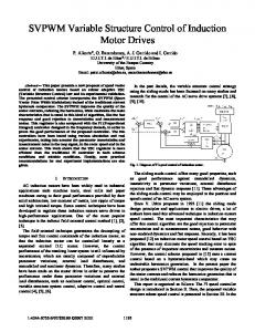
According to figure 4, K represents the system’s input and x the system’s output. The other adding terms in (15) are taken as system’s perturbations. With this representation of the system it is possible to regulate the scaled squared voltage x to a reference value
( )
x* = 0.5C vc*
2
and thus allowing to maintain
Fig. 5. Closed-loop poles locus for grid amplitude variations.
condition (6). With the control scheme depicted in figure 4 the system’s closed-loop transfer function can be derived as follows:
Notice that the designed controller depends upon the grid’s amplitude A. However, as depicted in Figure 5, a root locus analysis shows that the controller is robust to variations of A from its nominal value.
659
C. Steady State Analysis When the steady state is reached and assuming that the PV’s voltage and current vary very slowly with respect to T, equation (12) can be rewritten as: 2 L d ( Kv2 ) C dvc =− 2 + PPV − Kv2 2 dt 2 dt 2 2
(23)
In the steady state the generated power during one period T will be equal to the output power in the same time interval:
Ppv = Pout =
2P KA2 ⇒ K = PV 2 A2
(24)
As mentioned before, x represents the scaled squared voltage, therefore the following differential equation yields:
dx L K2 A2ω = PPV − 2 sin2ω t − KA2 sin2 ω t dt 2
(25)
Solving differential equation (25) and substituting the steady -state value of K:
x = α sin ( 2ω t + ϕ ) + x
*
PPV 2ω
vc = vc + vˆc d = d + dˆ
(26)
1
1
1
Where, vc is the reference value of the DC-link voltage, vˆc
Where
α =
have been proposed in order to reject these variations. The most common consists on adding an input capacitor in parallel to the solar cells, as in [11] where a method to size it efficiently is reported. Another approach consists on eliminating the oscillation in the input power by an appropriate control of the Boost converter. In [12] a sophisticated control principle was developed in order to allow the operation in the maximum power point without any power pulsation in the solar panel. The proposed MPPT follows the last approach. Equation (1) using the average model for the buck converter can be rewritten with u1=d1, where d1 represents the steady-state duty cycle. Therefore, it can be inferred that if the product vc (1− d1 ) is constant there won’t be a variation in the PV’s generated power. Therefore, a correcting factor for the boost’s duty cycle has been obtained in order to reject the 100Hz ripple, as follows: Defining the DC-link voltage (v C) and the Boost duty cycle (d1) as:
2 ⎛ A2 ⎛ 2L ω P ⎞ 1+ ⎜ 2 PV ⎟ ; ϕ = tan−1 ⎜ ⎜ 2L2ω PPV ⎝ ⎠ A2 ⎝
⎞ ⎟ ⎟ ⎠
represents the perturbation around vc , d1 is the commanded value given by table I which is updated every T G and dˆ1 is the variation around d1 . Therefore, in order to avoid variations in the PV generated power the following equation has to be fulfilled:
Notice that in the steady state the voltage in the DC link will present an oscillation of 100Hz from its reference value. From (26) it is possible to reach an expression from which the value of C can be minimized. According to (26), the
(
vc ⋅ (1 − d1 ) = vc ⋅ 1 − d1
* minimum value of x is x min = x − α . Applying condition (9)
( vc + vˆc ) ⋅ (1 − ( d1 + dˆ1 ) ) = vc ⋅ (1− d1 )
to the scaled squared voltage x:
x>
(
)
2 A 2C ⎛ 2 ⎞ ⎜1 + KωL ⎟ 2 ⎝ ⎠
(27)
C>
(
vc *2 − A 2 1 + Kω L22
)
(
vˆc ⋅ 1 − d1 dˆ1 = vc
(28)
)
(30)
TABLE I. HILL CLIMBING MPPT ALGORITHM
K[ n] − K[ n − 1] d1[ n − 1] − d1[ n − 2] V.
(29)
Finally, solving for dˆ1 yields:
Substituting (26) into condition (27) and solving for C:
2α
)
PROPOSED POWER SENSORLESS MPPT
The proposed MPPT is based on a sensorless MPPT control scheme presented by Kitano et al [10]. This algorithm relies on the fact that when the steady state is reached the DC-link voltage is kept constant due to the action of the inverter’s controller. Therefore, the generated power of the solar array and the regenerative power to the system side should be in balance. This will make the output current’s amplitude proportional to the PV’s generated power. Varying the boost’s duty cycle to maximize the current amplitude will result on a tracking of the PV’s MPP. A hill climbing algorithm was used in [10] to maximize the current amplitude with satisfactory results. A similar approach has been used in the proposed MPPT; nevertheless some modifications have been made in order to adapt it to the proposed system’s control scheme. Namely, how the current amplitude’s updating period will affect the algorithm. Since K is updated every TG seconds the MPPT will be affected by perturbations that occur within that timeframe. The climate variations are slower than TG but the ripple due to the 100Hz pulsation in the output power of the single-phase inverter won’t be rejected efficiently. From equation (26) it can be deduced that the DC-link voltage presents a 100Hz oscillation which will move the PV module from its maximum power point. Different approaches
VI.
d1[ n]
0
d1[ n − 1] + δ
SIMULATION RESULTS AND CONCLUSIONS
This section is devoted to verifying the proper operation of the designed power conditioning system which links a 2kW photovoltaic array to the utility grid. The values of the European utility grid (220@50Hz) were used and the solar array was modeled according to the PV’s electrical equations given in [3] and the parameters taken from General Electric®’s GEPV-110M solar module. In order to obtain a 2kW PV’s generated power, two subarrays of 8 GEPV-110-M module series string were connected in parallel. The parameters of one GEPV-110-M solar module are summarized in table II.
660
TABLE II. PV’ S MODEL PARAMETER
Cells in series 36 Cells in parallel 1 Short circuit current 7.4 A Open circuit voltage 21.6 V Temperature coefficient 3 mA/C Band Gap Energy (EGO) 1.106 eV Ideality factor for a p-n junction 2.46 Series Resistance 0.02 Ω Saturation current 5 mA A Matlab® simulation of the complete system with the controller of equation (22) and the proposed MPPT has been carried out using the following parameters: • L1=1mH, L2=2mH, C=2mF. • ZAD switching frequency = 25kHz • MPPT frequency = 100kHz The simulation has been done with a ODE5 Dormand-Prince fixed-step continuous solver with a step size of 1x10⁻⁶ s. Figure 6 shows the simulation results of the designed inverter when the solar radiation changes from 60mW/cm2 to 100mW/cm2 and then from 100mW/cm2 to 80mW/cm2. Notice that according to figure 6.a. the maximum power point is always reached after a smooth transient response and that the DC-link capacitor voltage reaches the commanded value of 450V. From figure 6.b it can be seen that the output current is in phase with the utility grid voltage. The scale factor K showed in figure 6.c also presents a stable response thus validating the obtained linear sampled data model. Finally, figure 7 validates the designed system in front of more realistic insolation data. The input solar radiation data corresponds to a 90-minutes sunny day fragment as depicted in figure 7.a. The resulting DC-link voltage, PV voltage, PV current, output current amplitude and PV power are shown in figure 7.b.
(b)
(c) Fig. 6. Simulation results. (a) DC-link voltage, PV voltage and PV output power. (b) Output voltage and current. (c) K scale factor.
REFERENCES [1]
[2]
[3] [4] (a)
[5]
[6] [7]
[8]
661
M. Calais, J. Myrzik, T. Spooner, V. G. Agelidis, “Inverter for Single-Phase Grid Connected Photovoltaic Systems – An Overview,” Power Electron. Spec. Conf., Vol. 4, pp. 1995-2000, Feb. 2002. D. Biel, G. Guinjoan, E. Fossas, J. Chavarria. “Sliding-Mode Control Design of a Boost–Buck Switching Converter for AC Signal Generation”, IEEE Trans. on Circuits and Systems. Vol.51, Iss8, pp. 1539-1551, Aug. 2004. C. Hua, J. Lin, C. Shen, “Implementation of a DSP -Controller Photovoltaic System with Peak Power Tracking,” IEEE Transactions on Industrial Electronics, Vol. 45, n1, Feb. 1998. J. Kassakian, M. Schlecht and G.Verghese, Principles of Power Electronics. Norwell, MA: Addison-Wesley, 1991,pp. 395-399. K. Mahabir, G.Verghese, V.J. Thottuvelli, and A. Heyman, “Linear averaged and sampled data models for large signal control of high power factor ac-dc converters”, in Power Electron. Special. Conf. Rec., 1990, pp.291-299. A. Mitwalli, S. Leeb, G. Verghese and V. Thottuvelil, “An adaptive digital controller for a unity power factor converter,” IEEE Trans. Power Electron., vol. 11, pp. 347-382, Mar. 1996. R. Ramos, D. Biel, E. Fossas and F. Guinjoan, “A FixedFrequency Quasi-Sliding Control Algorithm: Application to Power Inverters Design by Means of FPGA Implementation,” IEEE Trasn. Power Electron., vol. 18, no 1, pp. 344-355, Jan. 2003. M. Carpita and M. Marchesoni, “Experimental study of a power conditioning using sliding mode control,” IEEE Trans. Power Electron., vol. 11, no. 5, pp. 731-742, 1996.
Photovoltaic Source While Drawing Ripple-Free Current. Power Electron. Spec. Conf. 2002. pp. 1518-1522. [12] R. Schmidt, F. Jenni, J.Riatsch. Control of an Optimized Converter for Modular Solar Power Generation. -. IECON, 1994. pp. 479-484.
V.I. Utkin, Sliding mode and their applications in variable structure systems. Ed. Mir. Moscow, 1978. [10] T. Kitano, M. Matsui, D. Xu. Power Sensor-less MPPT Control Scheme Utilizing Power Balance at DC Link –System Design to Ensure Stability and Response -. IECON, 2001, pp. 1309-1314. [11] T. Brekken, N. Mohan, C. Henze, L. Moumneh. Utility-Connected Power Converter for Maximizing Power Transfer From a [9]
Fig. 7.a. Insolation of a sunny day
Fig. 7.b. Simulation results of 90-minutes sunny day fragment simulation
662