This article has been accepted for publication in a future issue of this journal, but has not been fully edited. Content may change prior to final publication. Citation information: DOI 10.1109/TIE.2017.2674600, IEEE Transactions on Industrial Electronics
1
Current Control of Grid-Connected Inverter with LCL Filter Based on Extended-State Observer Estimations Using Single Sensor and Achieving Improved Robust Observation Dynamics Baochao Wang, Member, IEEE, Yongxiang Xu, Member, IEEE, Zhaoyuan Shen, Jibin Zou, Senior Member, IEEE, Chaoquan Li and Hong Liu Abstract—In the context of distributed generation and renewable energy penetration towards smart grid, grid connected inverter with LCL filter has drawn many attentions, whose current control conventionally requires several sensors to realize active damping and grid synchronization. In this paper, a novel full status observation strategy based on extended state observer (ESO) is proposed using inverter current feedback only and without grid voltage sensor. The proposed observation strategy contains observation and transformation process. Unlike conventional Luenberger observer, by using ESO, the system parameters do not appear in observation process, thus the observer dynamics and parameter mismatch error can be separately handled, providing more robust observation dynamics during parameter variation. Parameter mismatch study was carried out, and it is found that purposely choosing the observer parameters smaller than the real value can achieve relatively low estimation error and a large adaption range for parameter variation. The proposed observation strategy is simple to implement, without the need of expert knowledge based parameter tuning such as pole placement. Experimental tests validated that the proposed observation based control is able to give satisfactory performance in both dynamic and steady states, as well as adaption for system parameter variation. Index Terms—Extended state observer, Observer dynamic decoupling, Parameter mismatch, Independent of expertise tuning, Grid connected inverter, LCL filter, Single sensor, Active damping, Grid synchronization Manuscript received May 30, 2016; revised September 26 and December 01, 2016; accepted December 21, 2016. This work was supported in part by the National Natural Science Foundation of China under Grant 51607045 and Grant 51437004, in part by the Fundamental Research Funds for the Central Universities under Grant HIT.NSRIF.201610, in part by the Heilongjiang postdoctoral Fund under Grant LBH-Z15067, and in part by the State Key Laboratory of Robotic and Systems (HIT) under Grant SKLRS201507B. C. Li is with Navigation and Control Institute, NORINCO,Beijing, China (
[email protected]). The other authors are with 3 different institutions of Harbin Institute of Technology (HIT), Harbin, China. Y. Xu, Z.Shen, J. Zou are with School of Electrical Engineering and Automation. H. Liu is with School of Mechatronics Engineering. J. Zou and H. Liu are with State Key Laboratory of Robotics and System (HIT). (
[email protected],
[email protected],
[email protected],
[email protected]) Baochao Wang is with State Key Laboratory of Robotics and System (HIT), and with School of Electrical Engineering and Automation, both in Harbin Institute of Technology, Harbin, China. (phone: +86 -451-86413613 ext 605; fax: +86-451-86413613 ext 600; e-mail:
[email protected] ).
I. INTRODUCTION ITH the development of renewable energy penetration, grid-connected LCL filter has drawn much attention for their higher attenuation ability, smaller volume and lower cost compared with conventional L filter. However, the inherent resonance problem of LCL filter has introduced more difficulties for grid-side current control. Due to resonance gain peak presented in frequency domain of LCL filter, both inverter and grid voltage harmonic component near resonance frequency can induce resonance in grid-side current. If ignoring resistance and frequency-dependent iron and copper losses, the gain could be infinite. However, it is worth noting that such infinite gain is not instantaneous, but integral with time, i.e. the resonance current amplitude gradually increases towards infinite under the persistent stimulation of the corresponding harmonic voltage. Thus, persistent current resonance must satisfy the following two conditions: (a) the voltage (grid or inverter) has persistent harmonic component near resonance frequency; (b) the system dynamic provide integral amplification at resonance frequency. Hence, the existing active damping techniques can be divided into two groups: to prevent condition (a) or to prevent condition (b). Techniques in the first group are mainly open-loop methods. Notch filter [1, 2], high pass filter [3] are often used to wipe out the persistent resonant harmonic component in inverter output voltage. However, this technique is not sufficiently effective on current resonance induced by grid voltage harmonics. Techniques in the second group are mainly closed-loop methods. They modify system dynamics by establishing feedbacks mechanism, such as virtual impedance, pole-placement, capacitor current feedback, etc. Virtual impedance methods are initiated from virtual resistance equivalent block diagram transformation [4]. Actually, virtual resistance can be hardly realized due to control delay, virtual impedance is recently reported to be more feasible, such as virtual RC [5] and virtual RL [6]. Pole placement usually requires all states measurements, recently grid voltage and grid current sensor based pole placement has been realized [7]. One of the most widely used techniques is to establish inner proportional feedback loop of capacitor current, the current can also be obtained by differentiation of capacitor voltage. Mathematically, capacitor voltage differentiation is
W
0278-0046 (c) 2016 IEEE. Translations and content mining are permitted for academic research only. Personal use is also permitted, but republication/redistribution requires IEEE permission. See http://www.ieee.org/publications_standards/publications/rights/index.html for more information.
This article has been accepted for publication in a future issue of this journal, but has not been fully edited. Content may change prior to final publication. Citation information: DOI 10.1109/TIE.2017.2674600, IEEE Transactions on Industrial Electronics
2 proportional to capacitor current, however, in discrete time and with the presence of noise, the differentiation requires more attention, lead-leg [8] and non-ideal integrator [9] are proposed to achieve better differentiation signal. It is also worth noting that the capacitor current inner loop feedback is equivalent to virtual resistor parallel with the capacitor [5]. The conventional grid current active damping using capacitor current feedback requires two current sensors and one grid voltage sensor. The current sensors measures grid current and capacitor current for active damping, and grid voltage must be measured for current phase synchronization and power factor control. Recently, research concern is moving towards active damping strategy with fewer sensors. One way is to transform the block diagram so that the capacitor current loop can be merged with grid current feedback, such as in [5] and [6]. The other way is to use the state space model and observers. In [10], Luenberger observer is used to estimate the capacitor current, which is used to pass virtual resistor to achieve active damping. Using converter current measurement, observer based pole-placement is obtained in [11]. However, although these techniques reduce the total number of sensors for state variables, the grid voltage still requires measurement, which results in an additional sensor. Several grid voltage sensorless control techniques have been reported in the literature [3, 12, 13]. In [3], by ignoring capacitor current, the capacitor voltage and grid current can be estimated through model calculation with inverter voltage and current. However, direct calculation from model does not provide good noise attenuation, and the assumption of ignoring capacitor current does not suite the case in which the impedance of the capacitor branch is not much higher than inductor branch. In [12], taking inverter current feedback only, Kalman filter is used to estimate the distorted grid voltage. A 14-states model, considering several grid harmonics are presented and used to estimate grid voltage, which is complicated. In [13], explicit model predictive control is proposed, in which separate state observer and grid estimator are used, and capacitor voltage is measured for a better dynamic performance. However, all the conventional observers or model-based methods requires expert knowledge for parameter tuning, such as pole placement, because real state variables are chosen for observation and system parameters are involved in the design process, which makes it difficult for a non-expert use or for adaption of a different configuration. In addition, the conventional observers use real plant model, the observer dynamics and parameter mismatch error are often coupled together and not drawing attention. Extended state observer (ESO) is one essential element in Active Disturbance Rejection Control (ADRC) [14], which has made a significant breakthrough that the observer variables can be chosen other than real state variables, and even the function of variables can be treated as extended variable, which provides more possibilities for observation and control. Recently, combinations of ESO with other controllers are also reported to improve control performance industrial and military applications [15-20], which mainly aim at handling external
disturbances. However, using ESO to extract both internal states and external disturbance without expertise parameter tuning, and make control based on the extracted information has not been explored so far. In this paper, by using ESO, a simple single sensor based current control for grid-connected inverter with LCL filter can be realized; neither capacitor current sensor nor grid voltage sensor is required for active damping or grid phase synchronization. The observation does not need expertise parameter tuning. The control is based on observation other than measurement, and the stability is proved by theoretical analysis and experimental results. Moreover, the proposed method separates observation dynamics and parameter mismatch error, which are often coupled in conventional observers, resulting in more robust adaption for parameter variation. The subsequent content is organized as follows: section II gives the system description, and then the proposed ESO implementation and corresponding analysis are given in section III. It is followed by experimental results in section IV, correspondingly. Section V gives a detailed discussion on dynamic performance, advantages over conventional Luenberger observer together with parameter mismatch influence and countermeasure. Finally, the conclusion is given in section VI. II. LCL–TYPE SINGLE-PHASE GRID-CONNECTED INVERTER DESCRIPTION
The grid-connected inverter with LCL filter is shown in Fig. 1. LI , R I , LG , RG and C are filter parameters, respectively inductance and resistance of inverter-side inductor, inductance and resistance of grid-side inductor, and filter capacitance. uDC , u I , u C and u G are respectively DC bus voltage, inverter output voltage, capacitor branch voltage and grid voltage, iI , iC and iG are inverter-side current, capacitor branch current and grid-connected current. V1 DC Source
V2
iI LI
RI
iG LG RG
uI
uC
iC uDC
V3
C
Grid
uG
V4
Fig. 1 Grid-connected inverter by LCL filter.
The block diagram of the filter can be represented as Fig. 2.
uG
uI
iI 1 LI s +RI
1 Cs
1 LG s RG
iG
uC Fig. 2 Block diagram of LCL filter.
The transfer function between iG and u I can be expressed as:
0278-0046 (c) 2016 IEEE. Translations and content mining are permitted for academic research only. Personal use is also permitted, but republication/redistribution requires IEEE permission. See http://www.ieee.org/publications_standards/publications/rights/index.html for more information.
This article has been accepted for publication in a future issue of this journal, but has not been fully edited. Content may change prior to final publication. Citation information: DOI 10.1109/TIE.2017.2674600, IEEE Transactions on Industrial Electronics
3 iG ( s ) 1 u I ( s ) LI LG Cs 3 ( RI LG RG LI )C s 2 ( RI RG C LI LG ) s ( RI RG )
(1)
where s is the Laplace operator. If ignoring the resistance in eq.(1), eq.(2) can be obtained. iG ( s ) 1 (2) 3 uI ( s ) LI LG Cs ( LI LG ) s The transfer function indicates that the system has resonance problem, which requires active damping technique for stable current control. Classic capacitor current feedback requires two current sensors for current measurements and one voltage sensor for grid voltage measurement. By the proposed control strategy in the following section, only inverter current measurement is used for both active damping and grid synchronization. III. PROPOSED FULL STATUS ESTIMATION BASED ON ESO AND CORRESPONDING CONTROL ALGORITHM WITH INVERTER SIDE CURRENT FEEDBACK ONLY
The overview of the proposed control scheme is shown in Fig. 3, which consists of four parts: ESO, transformation module, conventional active damping algorithms but based on estimation, the phase locked loop (PLL) for grid synchronization using estimated grid voltage. The proposed ESO takes the inverter current feedback and gives the estimation of a group of virtual variables [ z1 z2 z3 z 4 ] ' . Transformation module convert the output of
ESO to the estimations of real state variables [iˆI uˆ C iˆG ] ' and grid voltage uˆ G . The current estimations iˆI and iˆG are used for active damping, which is the conventional technique using capacitor current proportional feedback inner loop. The grid voltage phase is extracted by applying PLL to the estimated grid voltage uˆ G . Given desired amplitude I AMP , the grid current reference iG* is generated as in (3), which aims at unity power factor operation for maximum energy injection into the grid. It is worth noting that only inverter current is measured for full status estimation, but the control does not use this measured signal but pure estimations. LCL Filter
Power Stage
LI DC voltage source
LG
SPWMVSI
C
PWM
Amplitude Reference generator I
iG
iI
uPWM
GC ( s)
AMP
Phase
PLL
iˆC iˆI uˆC iˆG
HC
Transformation (Eq. 17,18)
uˆG
Inverter Compensation (Eq. 20)
uI z1 z z32 z3 z4
Current sensor
x1 ESO (Eq. 12)
Control board
Fig. 3. Proposed control scheme.
Grid
iG* I AMP sin( )
(3)
A. Extended State Observer Any arbitrary general 3rd-order system can be transformed in the following cascade integral form. x1 x2 x x 2 3 (4) x f ( x1 , x2 , x3 , u ) b0 u w 3 y x1
Where, x1 , x2 and x 3 are the state variables of the cascade integral form, f ( x1 , x2 , x3 , u ) represents the dynamics of the
system, which is the so-called “internal disturbance”, u is the control variable, y is the output variable, w is external
disturbance, b0 is the coefficient describing the influence from u to the cascade integral system. The relation can be expressed as in Fig. 4. w u
b0
1 s
x3
1 s
x2
1 s
x1
y
f ( x1 , x2 , x3 , u ) Fig. 4. Cascade integral form of any arbitrary 3-order system
By this cascade form, different systems at the same order can be expressed in a canonical form. The ESO does not distinguish “internal disturbance” or “external disturbance”, but treats them together as another state variable, which is the “overall disturbance”. For three order system, four order ESO must be used with total disturbance as another state variable. The four order ESO can be expressed as follows. e z1 x1 z z b e 2 1 1 (5) z2 z3 b2 e z z b u b e 4 0 3 3 z4 b4 e In this form, ESO takes the input value x1 and gives the estimation variables z 1 , z 2 , z 3 , z 4 , which are respectively the estimation of x1 , x2 , x3 and the overall disturbance. By selecting the feedback coefficients b1 , b2 , b3 , b4 properly, the estimation error converges to sufficiently small value. It can be seen that by using cascade integral form, the system parameters does not appear in the estimation, but acts only in the disturbance, so that the estimation can be designed without dependence on system parameter, and thus provides strong robustness for observer dynamics, which will be further discussed in Section V. B. State variable reconstruction based on ESO With the output of ESO, i.e., all states as well as disturbance, the full status of LCL filter can be obtained by only one measurement and internally know control signal, the procedure
0278-0046 (c) 2016 IEEE. Translations and content mining are permitted for academic research only. Personal use is also permitted, but republication/redistribution requires IEEE permission. See http://www.ieee.org/publications_standards/publications/rights/index.html for more information.
This article has been accepted for publication in a future issue of this journal, but has not been fully edited. Content may change prior to final publication. Citation information: DOI 10.1109/TIE.2017.2674600, IEEE Transactions on Industrial Electronics
4 is as follows: The state-space description of the LCL converter is as in (6). 1 diI dt L (uI uC iI RI ) I duC 1 (iI iG ) (6) C dt diG 1 (uC uG iG RG ) dt L G The equations can be written as x1 k5 x1 k 4 x2 k 4 u I x2 k3 x1 k3 x3 x k x k x k u 2 2 1 3 2 G 3 Where, x1 iI , x2 uC , x3 iG , k1 k3
e1 z1 x1 e1 e2 b1 e1 (13) e2 e3 b2 e1 e e b e 4 3 1 3 e4 b4 e1 According to eq. (13), the transfer function between disturbance estimation error e4 and overall disturbance
dOVERALL x4 can be derived as
s 4 b1s 3 b2 s 2 b3 s dOVERALL ( s) (14) s b1s 3 b2 s 2 b3 s b4 Since the ESO is based on canonical cascade integral model, which is order-dependent instead of precise-model-dependent, the coefficients can be chosen according to priori-tuned parameter rules, such as ‘Fibonacci sequence method’ proposed in [21]. Specifically, for three-order system, 1 1 2 5 , b3 , b4 . b1 , b2 (15) 2 (3h)h h (8h) h (13h)3 h e4 ( s )
(7)
RG 1 , k2 , LG LG
R 1 1 k5 I . , k4 LI LI C
By substituting x1 x1 x2 k5 x1 k4 x2 k4 uI 2 x3 (k5 k3 k4 ) x1 k4 k5 x2 k3 k4 x3 k4 k5 uI k4 uI the system can be presented in cascade integral form, as x1 x2 x2 x3 x3 f ( x1 , x2 , x3 , u I ) k 2 k3 k 4 uG k 2 k3 k 4 u I
(8)
(9)
Where x1 , x2 , x3 are cascade state variables, and
f ( x1 , x2 , x3 , uI ) 1 x1 2 x2 3 x3 k1k4uI k4uI 1 (k1k3k4 k2 k3k5 ) (10) 2 (k1k5 k2 k3 k3k4 ) 3 (k1 k5 ) Taking the overall disturbance in (9) as the extended state variable, and denoting the overall disturbance as dOVERALL f ( x1 , x2 , x3 , u I ) k2 k3k4uG (11) The linear form ESO is used for this application, which is expressed as follows. e z1 x1 z1 z2 b1 e (12) z2 z3 b2 e z z k k k u b e 4 2 3 4 I 3 3 z4 b4 e Denoting the estimation error as e1 z1 x1 , e2 z2 x2 , e3 z3 x3 and e4 z4 x4 , the equation of estimation error can be derived as:
4
Where h is dependent on the desired bandwidth and can be set as the sampling time interval. Solving eq. (8), the cascade state variables can be converted to normal state variables as: x1 x1 (16) x2 ( k5 x1 x2 k 4 u I ) / k 4 x ( k k x k x x k u ) / k k 3 4 1 5 2 3 4 I 3 4 3 Thus, with the estimation results of ESO, The estimation of the original state variables can be derived from the output of ESO as iˆI z1 (17) uˆC ( k5 z1 z 2 k 4 u I ) / k 4 ˆ iG ( k3 k 4 z1 k5 z 2 z3 k 4 u I ) / k3 k 4 It can be seen that the system parameters do not appear in ESO design, and they are only used in the simple algebraic transformation in (17), where only addition and multiplication are involved. Thus, for the system, both observer parameter or transformation equation can be fixed, so that expertise parameter tuning such as pole placement is avoided, which results in easier observation design and better adaption for different system configurations. C. Grid voltage reconstruction based on ESO and phase synchronization To operate the inverter without grid voltage sensor, the grid voltage must be obtained. The forth output of ESO z 4 is the overall disturbance and contains the grid voltage information and internal disturbances. According to eq. (10) and eq. (11), the estimation of grid voltage can be obtained as follows: z f ( z1 , z2 , z3 ,uI ) uˆG 4 (18) k 2 k3 k 4 By using ESO, the grid voltage, which is external input other than real-state-variable, are treated equally as part of the overall disturbance of ESO, and can be obtained through simple
0278-0046 (c) 2016 IEEE. Translations and content mining are permitted for academic research only. Personal use is also permitted, but republication/redistribution requires IEEE permission. See http://www.ieee.org/publications_standards/publications/rights/index.html for more information.
This article has been accepted for publication in a future issue of this journal, but has not been fully edited. Content may change prior to final publication. Citation information: DOI 10.1109/TIE.2017.2674600, IEEE Transactions on Industrial Electronics
5 algebraic calculation as well. To get grid voltage phase angle and to attenuate the high-order harmonics in grid voltage estimation, a PLL with orthogonal signal generator is used [22], which is able to provide filtering without delay. D. Active damping To damp the resonance, conventional capacitor current feedback technique is used, as shown in Fig. 3. The current controller is PI controller, which can be expressed as: K (19) GC ( s ) K P I s The output of the controller is denoted as uPWM , ranging -1~1. Using bipolar PWM modulation strategy and neglecting voltage drop and dead time of switching component, the relation between inverter output and controller output is as: u I u PWM u DC (20)
(27) uI ( s ) [(iG* HiˆG )Gc ( s ) H C (iˆc )]GINV ( s ) H is sampling gain, which takes the value 1. Substituting eq. (21) and eq. (22) into eq. (27), the transfer function between iI , iG* and u I can be obtained as follows: GINV ( s )Gc ( s ) uI (s) iG * ( s ) 1+GINV ( s )[Gc ( s ) HGu iˆ ( s ) H C Gu iˆ ( s )] I
iI iG
iˆC ( s ) Gi
I
iˆC
I
iˆC
( s )u I ( s )
(22)
1 LG s RG
iˆG
H (s)
GC ( s )
be expressed by iG and uG in s-domain as follows iI ( s ) GiG iI ( s )iG ( s ) GuG iI ( s )u G ( s )
(29)
u I ( s ) GiG -u I ( s )iG ( s ) GuG -u I ( s )u G ( s )
(30)
GiG iI (1 LG Cs 2 )
(31)
Where,
G iG -u I ( s ) L I LG Cs ( R I LG RG L I )C s 3
+(k3 k 4 b3 k5 b4 ) s k3 k 4 b4 }
s k3
1 4 3 k3 k 4 (s b1s b2 s 2 b3 s b4 )
{(b1 1)s 5 [ k5 (b1 1) (b2 1)]s 4
G uG -u I ( s ) L I Cs 2 R I Cs 1
(33) (34)
Substituting eq.(29) and eq. (30) into eq. (28), the grid injected current iG can be expressed by reference command iG * and grid voltage uG as follows:
( k3 k 4 b1 k5 b2 b3 ) s 3 ( k3 k 4 b2 k5 b3 b4 ) s 2
GuI iˆG ( s )
(32) 2
( R I RG C LI LG ) s ( R I RG )
(23)
{(b1 1)s 5 [ k5 (b1 1) (b2 1)]s 4
iG
On the other hand, according to eq. (6), both uI and iI can
G uG iI Cs
1 k3 k 4 (s 4 b1s 3 b2 s 2 b3 s b4 )
iG
H C ( s)
GINV ( s )
iI ( s )
Fig. 5. Block diagram of the closed loop system.
iˆ ( s ) GiI iˆG ( s ) G iI ( s )
GiI iˆC ( s )
iˆC
GuI iˆC ( s )
GiI iˆG ( s )
C
GuI -iˆG ( s )
Where,
1 iI 1 LI s +RI Cs
I
(28)
uG
Gi iˆ ( s )
uI
C
1+GINV ( s )[Gc ( s ) HGuI iˆG ( s ) H C GuI iˆC ( s )]
u I iG
( s )iI ( s ) Gu
I
uC
The capacitor current feedback coefficient H C determines the desired damping ratio. This coefficient as well as the grid current controller parameter can be tuned according to bode diagram or root locus analysis, such as in [23]. E. Stability and analysis After applying the ESO, the control is based on the observation results, and the observer dynamics should be considered to evaluate the system performance, it is analyzed as follows. According to eq. (12) and eq. (17) the transfer function between current estimation results [ iˆG iˆC ] and the sampled current i I can be derived as: iˆG ( s ) G ˆ ( s )iI ( s ) G ˆ ( s )uI ( s ) (21)
G
GINV ( s )[Gc ( s ) HGiI iˆG ( s ) H C GiI iˆC ( s )]
iG ( s ) Gi
(24)
G
*
iG
( s )iG * ( s )+GuG iG ( s )uG ( s )
(35)
Where, (25)
( k5 b2 b3 ) s 3 ( k5 b3 b4 ) s 2 +k5 b4 s}
s GuI iˆC ( s ) (26) k3 Based on the analysis above, the block diagram of the closed loop system can be represented as Fig. 5, and the input voltage of LCL filter u I can be expressed as:
Gi
G
*
iG
(s)
G INV ( s )Gc ( s ) 1+GINV ( s )[Gc ( s ) HGuI iˆG ( s ) H C GuI iˆC ( s )] GiG -uI ( s )
GINV ( s )[Gc ( s ) HGiI iˆG ( s ) H C GiI iˆC ( s )]
1+GINV ( s )[Gc ( s ) HGuI iˆG ( s ) H C GuI iˆC ( s )]
(36) GiG iI ( s )
G INV ( s )[Gc ( s ) HGiI iˆG ( s ) H C GiI iˆC ( s )] Gu i ( s ) 1+ G INV ( s )[Gc ( s ) HGu I iˆG ( s ) H C Gu I iˆC ( s )] G I GuG iG ( s ) (37) G INV ( s )[Gc ( s ) HGiI iˆG ( s ) H C GiI iˆC ( s )] GiG -u I ( s ) GiG iI ( s ) 1+ G INV ( s )[Gc ( s ) HGu I iˆG ( s ) H C Gu I iˆC ( s )] GuG -u I ( s )
Selecting a set of parameter K P 10 , K I =2000 and H C =0.4 according to the traditional control strategy parameter
0278-0046 (c) 2016 IEEE. Translations and content mining are permitted for academic research only. Personal use is also permitted, but republication/redistribution requires IEEE permission. See http://www.ieee.org/publications_standards/publications/rights/index.html for more information.
This article has been accepted for publication in a future issue of this journal, but has not been fully edited. Content may change prior to final publication. Citation information: DOI 10.1109/TIE.2017.2674600, IEEE Transactions on Industrial Electronics
6
-1
Imaginary Axis(seconds )
tuning process, such as in [23]. With the selected parameters, the pole and zero map of the closed system was presented in Fig. 6, the closed loop bode diagram with both estimated variables feedback and measured variables feedback was presented in Fig. 7, where the subscript ‘EST’ indicates the system with estimated variables feedback, while the subscript ‘MES’ indicates the system with measured variables feedback. Fig. 6 and Fig.7 represent the relation of iG to iG* Fig. 6 shows that for closed loop control, all the pole of the control using estimated variables feedback are located on the left half plane, and the dominant poles are very close to the those of closed-loop control with measured variables feedback. Fig. 7 presents that both the magnitude-frequency curves and phase-frequency curves are almost the same for closed loop control whether using estimations or measurements. Therefore, the closed system with estimated variables feedback is stable in time domain and ought to have similar dynamic response compared to the closed system feedback with measured variables. Pole EST Zero EST Pole MES Zero MES 0.54
6000 4000 2000 0 -2000 -4000 -6000
0.3
0.4
0.21
0.06 6e+03 5e+03 4e+03 3e+03 2e+03 1e+03
0.13
0.7 0.9
1e+03 2e+03 3e+03 4e+03 5e+03 6e+03 0.06
0.9 0.7
-6000
0.54
-5000
0.3
0.4
-4000
-3000
0.21
-2000
0.13
-1000
Fig. 6. Pole and zero map of the closed loop system
Phase (rad/s) Magnitude (dB)
AC voltage source
DC voltage Source
Fig. 8. Photograph of the experimental setup. TABLE І SYSTEM PARAMETERS Symbol
60V
uG
Grid voltage
40Vpeak/50Hz
LI
Inverter-side inductance
4.14mH
RI
Internal resistance of inverter-side inductor Capacitor
19.3µF
Grid-side inductance
5.16mH
Internal resistance of inverter-side inductor
0.095Ω
Switching frequency
10KHz
RG
EST MES
1
2
10
3
10
4
10
5
10
Frequency (rad/s)
6
10
0.11Ω
TABLE II THE PARAMETERS OF CONTROLLER AND ESO Symbol
10
Value
DC bus voltage
fC
0 -50 -100 -150 -200 0 -90 -180 -270
Quantity
uDC
C LG 0
Real Axis (seconds-1)
relating to the experimental platform is given in Table I. The parameters of controller and ESO are as given in Table II.
7
10
Fig. 7. Bode diagram of the closed loop system.
IV. EXPERIMENTAL RESULTS
The proposed ESO based full status estimation and corresponding control strategies are tested with our experimental platform. A. Experimental Setup The photograph of the experiment platform is shown in Fig. 8. Grid is emulated by a programmable AC voltage source (Chroma 61511). The inverter power stage uses IGBT power module by Infineon (FS30R06W1E3). The control scheme is implemented in DSP TMS320F28069. The switching frequency is set to 10 kHz. The control and measurement frequency are the same as switching frequency. The parameters
Description
Value
h b1
Sampling time interval
1104
First coefficient of ESO
1104
b2
Second coefficient of ESO
3.3 107
b3
Third coefficient of ESO
3.131010
b4
Forth coefficient of ESO
2.281013
HC
Capacitor current feedback coefficient
0.4
KP
Proportional gain of controller
9
KI
Integration gain of controller
1800
B. Experimental Results of state variable reconstruction and grid voltage estimation During the test, the voltage signals are sensed by hall-effect voltage transducer (LV25-P). The current signals are sensed by hall-effect current transducer (CASR6-NP). Because the observation results in DSP cannot be displayed by an oscilloscope, for synchronized comparison with measurements, the observation results calculated in DSP are sent to PC through JTAG together with DSP measured signals at the same instant. Low pass digital filters with cut off frequency of 1KHz were
0278-0046 (c) 2016 IEEE. Translations and content mining are permitted for academic research only. Personal use is also permitted, but republication/redistribution requires IEEE permission. See http://www.ieee.org/publications_standards/publications/rights/index.html for more information.
This article has been accepted for publication in a future issue of this journal, but has not been fully edited. Content may change prior to final publication. Citation information: DOI 10.1109/TIE.2017.2674600, IEEE Transactions on Industrial Electronics
7 i
I_MES
i
i
I_EST
60 I_ERR
3 0 -3
-60 0
0.04
(a) Inverter-side current 60
9 C_ERR
G_MES
u
G_EST
i
6
G_MES
i
G_EST
i
G_ERR
3 0 -3 -6
0.01
0.02 Time (s)
0.03
-9 0
0.04
0.01
0.02 Time (s)
0.03
0.04
(c) Grid-side current 8
u
MES
G_ERR
EST
ERR
6
20
Phase (rad)
Voltage (V)
u
(b) Capacitor branch voltage u
40
C_EST
-20 -40
0.03
u
0
-9 0
0.02 Time (s)
C_MES
20
-6 0.01
u
40 Voltage (V)
Current (A)
6
Current (A)
9
0 -20
4 2
-40
0
-60 0
-2 0
0.01
0.02 Time (s)
0.03
0.04
(d) Grid voltage
0.01
0.02 Time (s)
0.03
0.04
(e) Grid voltage phase
Fig. 9. Experimental comparison between measurements and ESO based estimations: (a) Inverter-side current; (b) Capacitor branch voltage; (c) Grid-side current; (d) Grid Voltage; (e) Grid voltage phase
applied to the measured signals and estimation signal for noise attenuation. In all the measured signals ( iI , uC , iG and uG ), only inverter-side current iI is used for ESO estimation. The other measured signals are only used for comparison with the estimation results. Fig. 9 shows the experimental results waveforms of state variables and grid voltage reconstruction based on ESO, where the subscript ‘MES’ indicates the signals measured by the sensors, while the subscript ‘EST’ indicates the estimated variables. Fig. 9 (a)-(c) show that the state variable estimations are consistent with the measurements, there are acceptable errors caused by uncertain disturbance and sensor errors. Fig. 9 (d)-(e) show that even with high-order harmonics in grid voltage estimation, the grid phase maximum estimation error is 2.04% after wrapping the error with the period of 2 , which does not affect the grid synchronization or power factor control. . C. Experimental Results of current control based on pure estimations.
Based on ESO, the full status estimations are used for grid-injection current control with conventional active damping technique. It is worth noting that the following steady and transient results are all based on pure estimations throughout the test, where the inverter current is merely measured for full status estimation but never used in control. The ESO based observation algorithm execution time is 0.87us, using the 32-bit floating point MCU with 90MIPS. Fig. 10 shows the transient waveforms of grid-connected current after starting up with 6A peak current reference. By the proposed control strategy based on pure estimations, the system is able to self-start and converge after one grid period. Unlike conventional measurement-based control, the estimation-based control cannot give as good operation in the first period, because the estimations do not have any information, neither grid phase nor current value, until startup. However, the current
can still be maintained converging during the first period after startup. One and a half period after startup, the current is stable in phase, signifying the estimations of both state variables and grid voltage can converge successfully during transients, as well as PLL. The grid injection current is well damped and smooth. Fig. 11 presents transient waveforms during resonance and damping transients, which demonstrates the robustness of this method during resonance. At the beginning, HC is with the value that purposely detuned, in order to get the current resonance. Then at the falling edge of the coefficient change signal, HC is changed to the normal value. It can be seen that not only resonance can be effectively damped after one half period, but also the pure-estimation based control is stable throughout current resonance period and damping transients. Fig. 12 shows the transient waveforms when the reference current amplitude steps from 4A to 6A. It can be seen that the grid current is able to track the reference change within 4ms, and the transient overshoot about 13%. The control is stable during the transients. Fig. 13 shows steady-state waveforms. The grid injection current can be controlled in phase with the grid voltage, which aims at improving energy efficiency by unity power factor operation. The waveform is sinusoidal and stable, which gives satisfactory current injection performance. The steady state current THD is 3.8%. Fig. 14 shows steady-state waveforms under distorted grid voltage with voltage THD of 2.91%. The steady state current THD is about 4.46%. V. DISCUSSIONS A. Dynamic performance analysis
The transient performance relies on two aspects: the PLL transients and the observation transients.
0278-0046 (c) 2016 IEEE. Translations and content mining are permitted for academic research only. Personal use is also permitted, but republication/redistribution requires IEEE permission. See http://www.ieee.org/publications_standards/publications/rights/index.html for more information.
This article has been accepted for publication in a future issue of this journal, but has not been fully edited. Content may change prior to final publication. Citation information: DOI 10.1109/TIE.2017.2674600, IEEE Transactions on Industrial Electronics
8
Coefficient change signal
Start up signal
uG
iG
iG
Fig. 10. Transient waveforms of startup.
Fig. 11. Waveforms during resonance and damping transients by changing the capacitor current estimation feedback coefficient HC. iG uG
Fig. 13. Steady state waveforms
grid phase
)
Fig. 17. Capacitor current estimation dynamics during startup with 5A peak current.(Signals: purple
iG
uG
Fig. 12. Transient waveforms when grid current reference steps from 4A to 6A.
iG uG
Fig. 14. Steady state waveforms with distorted grid voltage
Fig. 15. PLL startup tracking dynamics with 5A peak current.(Signals: red
uˆG , green uG , purple
Reference change signal
uG
iC ,red iˆC )
The experimental PLL transients are given in Fig. 15. It can be seen that the phase is able to converge within one period. The signals are realized by D/A of the MCU emulated by 1MHz PWM passing through a low pass RC filter with the time constant of 0.0001 ( R 1k, C 0.1uF ). The startup instant is at 40ms in the figure, triggered by external source.
Fig. 16. Grid current and voltage estimation dynamics during startup with 5A peak current.(Signals: purple iG ,red iˆG , green uG , blue uˆG )
Fig. 18. Startup current oscillation reduction with lower current reference
Grid current and voltage estimation during startup transient is given in Fig. 16. The capacitor current estimation during startup is in Fig. 17. It can be seen the states can converge very quickly. As iˆC is calculated using iˆG , so iˆG estimation error results in amplitude error iˆC . For high frequency oscillation in
0278-0046 (c) 2016 IEEE. Translations and content mining are permitted for academic research only. Personal use is also permitted, but republication/redistribution requires IEEE permission. See http://www.ieee.org/publications_standards/publications/rights/index.html for more information.
This article has been accepted for publication in a future issue of this journal, but has not been fully edited. Content may change prior to final publication. Citation information: DOI 10.1109/TIE.2017.2674600, IEEE Transactions on Industrial Electronics
IEEE TRANSACTIONS ON INDUSTRIAL ELECTRONICS
iˆC , they are in phase with the real oscillations, which guarantees the active damping works well. During the experiment, the iˆC amplitude error does not have obvious influence on grid current control. One possible reason is that iC is quite small (about 0.4A for 5A grid peak current injection), and such low frequency amplitude error can be easily compensated by the PI controller. Compared with the state convergence, PLL phase response is slower. Thus, to further reduce the negative impact of phase error during the startup period, the current injection reference for startup can be set to smaller value to avoid large current oscillations for startup. Fig. 18 gives the startup current with 1A current peak reference, and current overshoot during startup is largely reduced compared with Fig. 10.
B. Advantages over conventional Luenberger observer When using observers, final observation errors are affected by two factors: observer dynamics and model-mismatch error. Using the proposed ESO based method, the observation process does not rely on system parameters, and the above two factors can be decoupled. For conventional Luenberger observer, the observer parameters are calculated by pole placement depending on parameters. When there is model-mismatch, both observation dynamics deviation and model mismatch error will occur, as they are coupled together. Fig. 19 gives the coefficients of conventional Luenberger 4 observer for two cases of placing the poles as s with
10000 . The difference is one case use real value of LI in the observer, while the other uses 0.5LI . It can be seen that the coefficients have large difference, signifying observer dynamic are largely affected by parameter variation.
Fig. 19. Luenberger observer four coefficients for different parameters.
Fig. 20 shows experiment comparisons for ESO based observation and conventional Luenberger observer for parameter mismatch with 0.5LI. Both observer works well for the case without parameter variation, as in Fig. 20 (a) and (b). When with parameter variation of 0.5LI, ESO performance remains almost the same, but Luenberger observer dynamic are changed, suffering from high frequency oscillations in both grid current and grid voltage estimations, which result in control oscillation and failure, as in Fig. 20 (c) and (d).
(a) ESO using LI
(b) Luenberger observer using LI
(c) ESO using 0.5LI
(d) Luenberger observer using 0.5LI. Fig. 20. Different observer based control startup transients with 1A grid current reference for parameter mismatch. (Signals: purple iG ,red iˆG , green uG , blue uˆG )
Thus, by using the proposed ESO based observation, the observation dynamics and model mismatch error can be decoupled, offering advantages of robust observation dynamics. C. Parameter mismatch influence and countermeasure Model parameter mismatch error is unavoidable for observations because of the must-use of system model. However, it can be maintained relatively low by proper countermeasure. By exhaustive case studies, it is found that iˆG is mainly influenced by C, uˆG is mainly influenced by LG and uˆC is mainly influenced by LI. Fig. 21 gives the LG variation influence on uˆG for 5A peak current output. The variation range is from 0.01 to 10 times of the real value. It can be seen parameter variation on the left side can result in lower error levels for a large range. A conclusion can be made that when the parameters cannot be set to real value, purposely choosing the estimation parameters smaller than the real value can achieve relatively low estimation error in a large parameter variation range. When LG changes from 0.01 times to the real value, the amplitude percentage error and absolute phase error of uˆG can remain within 2% and 11.5° respectively. 150 120 90 60 30 0 -2 10
10
-1
10
0
10
1
80 70 60 50 40 30 20 10 0 -2 10
10
-1
10
0
10
1
(a) amplitude percentage error (b) absolute phase error in degree Fig. 21. The LG variation influence on uˆG
For other parameters, the conclusion is the same. For
0278-0046 (c) 2016 IEEE. Translations and content mining are permitted for academic research only. Personal use is also permitted, but republication/redistribution requires IEEE permission. See http://www.ieee.org/publications_standards/publications/rights/index.html for more information.
This article has been accepted for publication in a future issue of this journal, but has not been fully edited. Content may change prior to final publication. Citation information: DOI 10.1109/TIE.2017.2674600, IEEE Transactions on Industrial Electronics
IEEE TRANSACTIONS ON INDUSTRIAL ELECTRONICS
example, when C varies from 0.01 times to the real value, the amplitude percentage error and the absolute phase error of iˆG are within 1.1% and 2.5°. Fig. 22 shows the experiment validation of LG parameter variation on uˆG . The above influence trend can be reflected in experiment test, although the estimation error cannot match exactly the theoretical value as also affected by many other factors. For steady state, estimations using smaller value are still relatively good for grid synchronization, while estimations using larger value result in obvious observation error and oscillations. For transient performance, smaller value is always able to maintain stable startup performance, while larger values gives more oscillations in uˆG and can cause occasional startup failure. It can be seen the smaller value is also able to maintain stable dynamic performance. The results validate the feasibility of purposely choosing the estimation parameters smaller than the real value, to achieve relatively low estimation error in a large variation range. It is the same case for other parameters as C and LI. By this countermeasure, the observation can also adapt a large range of parameter variation with relatively low error level.
(a) using LG 0.1mH (about 1/60 of ((b) using LG 15mH (about 3 times of the real value) in transformation the real value) in transformation Fig. 22. Experimental validation of the LG variation influence on uˆG . (Signals: purple iG ,red iˆG , green uG , blue uˆG )
VI. CONCLUSION
In this paper, a novel full status observation strategy based on ESO is proposed for current control of grid connected inverter using inverter current feedback only and without grid voltage sensor. Unlike conventional Luenberger observer, by using ESO, the observer dynamics and parameter mismatch error can be separately handled, which provided more robustness observation dynamics during parameter variation. In addition, a parameter mismatch study was carried out, the feasibility of purposely choosing the observer parameters smaller than the real value to achieve relatively low estimation error and a large parameter variation adaption range is validated. Thus, the ESO based observation strategy can be generalized to replace classic Luenberger observer for better dynamic performance and parameter mismatch adaption. The overall observation is quite simple, does not require parameter tuning, and thus is ideal for non-expert use or for adaption of different configurations. Based on ESO and using single sensor, not only real state variables and external grid voltage can be estimated at the same time, but also the observation process is simplified in such a way: the system
parameters do not appear in observer design so that complex calculation such as pole placement can be avoided, and the system parameters are only used in simple algebraic transformation only including addition and multiplication, which results in easier observation design and better adaption for different system configurations. Based on proposed observation, stable grid injection current can be well controlled, where grid synchronization as well as active damping is realized. Experimental tests validated that the estimation based control is able to give satisfactory performance in both dynamic and steady states, as well as adaption for parameter variation. REFERENCES [1] J. Dannehl, M. Liserre, F. W. Fuchs, "Filter-based active damping of voltage source converters with LCL filter," Industrial Electronics, IEEE Transactions on, vol. 58, DOI 10.1109/TIE.2010.2081952, no. 8, pp. 3623-3633, 2011. [2] R. Pena-Alzola, M. Liserre, F. Blaabjerg, M. Ordonez, T. Kerekes, "A self-commissioning notch filter for active damping in a three-phase LCL-filter-based grid-tie converter," Power Electronics, IEEE Transactions on, vol. 29, DOI 10.1109/TPEL.2014.2304468, no. 12, pp. 6754-6761, 2014. [3] M. Malinowski S. Bernet, "A simple voltage sensorless active damping scheme for three-phase PWM converters with an LCL filter," Industrial Electronics, IEEE Transactions on, vol. 55, DOI 10.1109/TIE.2008.917066, no. 4, pp. 1876-1880, 2008. [4] P. A. Dahono, "A control method to damp oscillation in the input LC filter," in Power Electronics Specialists Conference, 2002. pesc 02. 2002 IEEE 33rd Annual, vol. 4, DOI 10.1109/PSEC.2002.1023044, pp. 1630-1635, 2002. [5] X. Wang, F. Blaabjerg, P. C. Loh, "Virtual RC damping of LCL-filtered voltage source converters with extended selective harmonic compensation," Power Electronics, IEEE Transactions on, vol. 30, DOI 10.1109/tpel.2014.2361853, no. 9, pp. 4726-4737, Sep 2015. [6] X. Wang, F. Blaabjerg, P. Loh, "Grid-current-feedback active damping for LCL resonance in grid-connected voltage source converters," Power Electronics, IEEE Transactions on, vol. 31, DOI 10.1109/TPEL.2015.2411851, no. 1, pp. 213-223, 2016. [7] C. A. Busada, S. Gomez Jorge, J. A. Solsona, "Full-state feedback equivalent controller for active damping in LCL filtered grid connected inverters using a reduced number of sensors," Industrial Electronics, IEEE Transactions on, vol. 62, DOI 10.1109/TIE.2015.2424391, no. 10, pp. 5993-6002, 2015. [8] R. Pena-Alzola, M. Liserre, F. Blaabjerg, R. Sebastian, J. Dannehl, F. W. Fuchs, "Systematic design of the Lead-Lag network method for active damping in LCL-filter based three phase converters," Industrial Informatics, IEEE Transactions on, vol. 10, DOI 10.1109/TII.2013.2263506, no. 1, pp. 43-52, 2014. [9] Z. Xin, P. C. Loh, X. Wang, F. Blaabjerg, Y. Tang, "Highly accurate derivatives for LCL-filtered grid converter with capacitor voltage active damping," Power Electronics, IEEE Transactions on, vol. 31, DOI 10.1109/TPEL.2015.2467313, no. 5, pp. 3612-3625, 2016. [10] V. Miskovic, V. Blasko, T. M. Jahns, A. H. C. Smith, C. Romenesko, "Observer-based active damping of LCL resonance in grid-connected voltage source converters," Industry Applications, IEEE Transactions on, vol. 50, DOI 10.1109/TIA.2014.2317849, no. 6, pp. 3977-3985, 2014. [11] J. Kukkola M. Hinkkanen, "Observer-based state-space current control for a three-phase grid-connected converter equipped with an LCL filter," Industry Applications, IEEE Transactions on, vol. 50, DOI 10.1109/TIA.2013.2295461, no. 4, pp. 2700-2709, 2014. [12] B. Bolsens, K. De Brabandere, J. Van den Keybus, J. Driesen, R. Belmans, "Model-based generation of low distortion currents in grid-coupled PWM-inverters using an LCL output filter," Power Electronics, IEEE Transactions on, vol. 21, DOI 10.1109/TPEL.2006.876840, no. 4, pp. 1032-1040, 2006. [13] S. Mariethoz M. Morari, "Explicit model-predictive control of a PWM inverter with an LCL filter," Industrial Electronics, IEEE Transactions on, vol. 56, DOI 10.1109/TIE.2008.2008793, no. 2, pp. 389-399, 2009. [14] H. Jingqing, "From PID to Active Disturbance Rejection Control,"
0278-0046 (c) 2016 IEEE. Translations and content mining are permitted for academic research only. Personal use is also permitted, but republication/redistribution requires IEEE permission. See http://www.ieee.org/publications_standards/publications/rights/index.html for more information.
This article has been accepted for publication in a future issue of this journal, but has not been fully edited. Content may change prior to final publication. Citation information: DOI 10.1109/TIE.2017.2674600, IEEE Transactions on Industrial Electronics
IEEE TRANSACTIONS ON INDUSTRIAL ELECTRONICS
Industrial Electronics, IEEE Transactions on, vol. 56, DOI 10.1109/TIE.2008.2011621, no. 3, pp. 900-906, 2009. [15] L. Yongfu, Y. Bin, Z. Taixiong, L. Yinguo, C. Mingyue, S. Peeta, "Extended-State-Observer-based double-loop integral sliding-mode control of electronic throttle valve," Intelligent Transportation Systems, IEEE Transactions on, vol. 16, DOI 10.1109/TITS.2015.2410282, no. 5, pp. 2501-2510, 2015. [16] X. Wenchao, B. Wenyan, Y. Sheng, S. Kang, H. Yi, X. Hui, "ADRC with adaptive Extended State Observer and its application to air-fuel ratio control in gasoline engines," Industrial Electronics, IEEE Transactions on, vol. 62, DOI 10.1109/TIE.2015.2435004, no. 9, pp. 5847-5857, 2015. [17] G. Wang, Y. Wang, J. Xu, N. Zhao, D. Xu, "Weight-Transducerless rollback mitigation adopting enhanced MPC with Extended State Observer for direct-drive elevators," Power Electronics, IEEE Transactions on, vol. 31, DOI 10.1109/TPEL.2015.2475599, no. 6, pp. 4440-4451, 2016. [18] Y. Jianyong, J. Zongxia, M. Dawei, "Extended-State-Observer-Based output feedback nonlinear robust control of hydraulic systems with backstepping," Industrial Electronics, IEEE Transactions on, vol. 61, DOI 10.1109/TIE.2014.2304912, no. 11, pp. 6285-6293, 2014. [19] Y. Jianyong, J. Zongxia, M. Dawei, "Adaptive robust control of dc motors with Extended State Observer," Industrial Electronics, IEEE Transactions on, vol. 61, DOI 10.1109/TIE.2013.2281165, no. 7, pp. 3630-3637, 2014. [20] Z. Zheng, X. Dong, L. Jingmeng, X. Yuanqing, "Missile guidance law based on Extended State Observer," Industrial Electronics, IEEE Transactions on, vol. 60, DOI 10.1109/TIE.2012.2232254, no. 12, pp. 5882-5891, 2013. [21] H. Jingqing, "Parameters of the Extended State Observer and Fibonacci Sequence," Control Engineering of China, vol. 15, DOI 10.14107/j.cnki.kzgc.2008.s2.050, pp. 1-3, 2008. [22] M. Ciobotaru, R. Teodorescu, F. Blaabjerg, "A new single-phase PLL structure based on second order generalized integrator," in PESC '06,IEEE, DOI 10.1109/PESC.2006.1711988, pp. 1-6, 2006. [23] J. Dannehl, F. W. Fuchs, S. Hansen, P. B. Thogersen, "Investigation of active damping approaches for PI-based current control of grid-connected pulse width modulation converters with LCL filters," Industry Applications, IEEE Transactions on, vol. 46, DOI 10.1109/TIA.2010.2049974, no. 4, pp. 1509-1517, 2010. Baochao Wang (S’10-M’14) was born in Jinan, China. He received the B.S. and M.S. degrees from Harbin Institute of Technology (HIT), Harbin, China, in 2008 and 2010, respectively, and the Ph.D degree from University of Technology of Compiegne (UTC), Compiegne, France, in 2014, all in electrical engineering. Since 2014, he has been a Lecture in School of Electrical Engineering and Automation, HIT. He is also with State Key Laboratory of Robotics and System (HIT). His current research interests include PMSM drive and control, renewable energy integration and power quality.
Jibin Zou (SM’00) was born on January 19, 1957, in Heilongjiang Province, China. He received the M.S. and Ph.D. degrees in electrical engineering from the Harbin Institute of Technology, Harbin, China, in 1984 and 1988, respectively. Since 1985, he has been engaged in the research in electrical machines. He was with the University of Liverpool, Liverpool, U.K. as a Visiting Research Fellow for one year. He is now a Professor in the State Key Laboratory of Robotics and System and in School of Electrical Engineering and Automation, Harbin Institute of Technology. Prof. Zou is a senior member of the IEEE Magnetics society, since 2000. His current research interests include permanent-magnet machine design and control. Chaoquan Li received B.S and Ph.D degrees, North China University of Water Resources and Electric Power, Zhengzhou, China, 2004 and Beijing Institute of Technology, Beijing, China, in 2011. Since 2011, he is with Navigation and Control Institute, NORINCO, as associate professor. His research interests focus on computer servo control systems based on DC motors, also include the sensor technology and its application on navigation and guidance control systems.
Hong Liu received B.S and Ph.D degrees from Harbin Institute of Technology, Harbin, China, in 1986 and 1993, respectively, Ph.D degrees in RWTH Aachen, Aachen, Germany and German Aerospace Center (DLR), Germany, in 1991 and 1993, respectively. From 1993 to 1999, he worked with Germany and German Aerospace Center (DLR) as Researcher and Advanced Researcher. Since 1999, he is with School of Mechatronics Engineering, Harbin Institute of Technology, as “Changjiang Scholor” award professor. His research interests focus on versatile robotic hand, also include the sensor technology and bio-machenical merging technologies.
Yongxiang Xu (M’03) was born in Guangxi Province, China, in 1977. He received the M.S. and Ph.D. degrees in electrical engineering from the Harbin Institute of Technology, Harbin, China, in 2001 and 2005, respectively. He is currently a Professor in School of Electrical Engineering and Automation, Harbin Institute of Technology, Harbin. His current research interests include permanent-magnet machine design and control. Zhaoyuan Shen received the M.S. degree from Harbin Institute of Technology, Harbin, China, in 2016. Since July 2016, he has been with CRRC Zhuzhou Institute CO.,LTD, Zhuzhou, China, as an Inverter Control Research Engineer. His research interests includes grid connected inverter control, asynchronous motor control and permanent magnet synchronous motor control.
0278-0046 (c) 2016 IEEE. Translations and content mining are permitted for academic research only. Personal use is also permitted, but republication/redistribution requires IEEE permission. See http://www.ieee.org/publications_standards/publications/rights/index.html for more information.