Boundary Element Methods - Springer Link

Chapter 4

Boundary Element Methods

In Chap. 3 we transformed strongly elliptic boundary value problems of second order in domains R3 into boundary integral equations. These integral equations were formulated as variational problems on a Hilbert space H : Find u 2 H W

b .u; v/ D F .v/

8v 2 H;

(4.1)

which, in the simplest cases, was chosen as one of the Sobolev spaces H s ./, s D 1=2; 0; 1=2. The functional F 2 H 0 denotes the given right-hand side, which, in the case of the direct method (see Sect. 3.4.2), may again contain integral operators. The sesquilinear form b .; / has the abstract form b .u; v/ D .Bu; v/L2 ./ with the integral operator Z .Bu/ .x/ D 1 .x/ u .x/ C 2 .x/

k .x; y; y x/ u .y/ dsy

x 2 a.e. (4.2)

Convention 4.0.1. The inner product .; /L2 ./ is again identified with the continuous extension on H s ./ H s ./. The coefficients 1 , 2 are bounded. For 1 D 0, a.e., one speaks of an integral operator of the first kind, otherwise of the second kind. In some applications the kernel function is not improperly integrable, and the integral is defined by means of a suitable regularization (see Theorem 3.3.22). The sesquilinear form in (4.1) associated with the boundary integral operator in (4.2) satisfies a G˚arding inequality: There exist a > 0 and a compact operator T W H ! H 0 such that 8u 2 H W jb .u; u/ C hT u; uiH 0 H j kuk2H :

S.A. Sauter and C. Schwab, Boundary Element Methods, Springer Series in Computational Mathematics 39, DOI 10.1007/978-3-540-68093-2 4, c Springer-Verlag Berlin Heidelberg 2011

(4.3)

183

184

4 Boundary Element Methods

The variational formulation (4.1) of the integral equations forms the basis of the numerical solution thereof, by means of finite element methods on the boundary D @, the so-called boundary element methods. They are abbreviated by “BEM”. Note: Readers who are familiar with the concept of finite element methods will recognize it here. One essential conceptual difference between the BEM and the finite element method is the fact that, in the BEM, the resulting finite element meshes usually consist of curved elements and therefore, in general, no affine parametrization over a reference element can be found. Primarily, we consider the Galerkin BEM, which is the most natural method for the variational formulation (4.1) of the boundary integral equation. In Sect. 4.1 we will describe the Galerkin BEM for the boundary value problems of the Laplace equation with Dirichlet, Neumann and mixed boundary conditions, all of which lead to boundary integral equations of the first kind with positive definite bilinear forms. We obtain quasi-optimal approximations and prove asymptotic convergence rates for the Galerkin BEM. In Sect. 4.2 we will then study Galerkin methods in an abstract form for operators that are only positive with a compact perturbation. We will also present a general framework for the convergence analysis of Galerkin methods. In Sect. 4.3 we will finally prove the approximation properties of the boundary element spaces.

4.1 Boundary Elements for the Potential Equation in R3 We will first introduce the Galerkin BEM for integral equations of the classical potential problem in R3 and derive relevant error estimates for the simplest boundary elements.

4.1.1 Model Problem 1: Dirichlet Problem Let R3 be a bounded polyhedral domain, the boundary D @ of which S consists of finitely many, disjoint, plane faces j , j D 1; : : : ; J : D JjD1 j . In the exterior C D R3 n we consider the Dirichlet problem u D 0 in C ;

(4.4a)

u D gD on ;

(4.4b)

ju.x/j D O.kxk1 / for kxk ! 1:

(4.4c)

In Chap. 2 (Theorem 3.5.3) we have shown the unique solvability of Problem (4.4).

4.1 Boundary Elements for the Potential Equation in R3

185

Proposition 4.1.1. For all gD 2 H 1=2 ./ Problem (4.4) has a unique solution u 2 H 1 .L; C / with L D . Proof. Theorem 2.10.11 implies solvability of the variational formulation the unique associated with (4.4) in H 1 L; C with L D . In Sect. 2.9.3 we have shown that the solution also solves (4.4a) and (4.4b) almost everywhere. Decay Condition: Theorem 3.5.3 provides us with the unique solvability of the boundary integral equation that results from (4.4) (with the single layer ansatz) in H 1=2 ./. The associated single layer potential is in H 1 L; C (see Exercise 3.1.14) and, thus, is the unique solution. Finally, in (3.22) we have shown that the single layer potential satisfies the decay condition (4.4c). We will now reduce (4.4) to a boundary integral equation of the first kind. We ensure that (4.4a), (4.4c) are satisfied by means of the single layer ansatz (see Chap. 3) Z '.y/ dsy ; x 2 C : (4.5) u.x/ D .S '/.x/ D 4 kx yk The unknown density ' from (4.5) is the solution of the boundary integral equation V ' D gD on (4.6) with the single layer operator Z .V '/.x/ WD

'.y/ dsy 4 kx yk

x 2 :

(4.7)

(4.6) defines a boundary integral equation of the first kind. The Galerkin boundary element method is based on the variational formulation of the integral equation. Instead of imposing (4.6) for all x 2 , we multiply (4.6) by a “test function” and integrate over . This gives us: Find ' 2 H 1=2 ./ such that Z Z

Z .V '/ dsx D

Z D

'.y/ dsy .x/dsx 4 kx yk

gD .x/ .x/ dsx

8 2 H 1=2 ./ :

(4.8)

For the Laplace operator we only consider vector spaces over the field R and not over C, so that in (4.8) there is no complex conjugation. 1 The “integrals” in (4.8) should be interpreted as duality pairings in H 2 ./ 1 H 2 ./ in the following way. For ' 2 H 1=2 ./ we have V ' 2 H 1=2 ./ and, by Convention 4.0.1, we can write (4.8) as Find ' 2 H 1=2 ./ W .V '; /L2 ./ D .gD ; /L2 ./

8 2 H 1=2 ./: (4.9)

186


The left-hand side in (4.9) defines a bilinear form b.; / on the Hilbert space H D H 1=2 ./ with b.'; / WD .V '; /L2 ./ ; (4.10) and the right-hand side defines a linear functional on H 1=2 ./ W F ./ WD .gD ; /L2 ./ :

(4.11)

Keeping the duality of H 1=2 ./ and H 1=2 ./ in mind, it follows from ! j .gD ; /L2 ./ j jF ./j sup kkH 1=2 ./ D kgD kH 1=2 ./ kkH 1=2 ./ 2H 1=2 ./nf0g k kH 1=2 ./

that F is continuous on H 1=2 ./. For sufficiently smooth functions '; in (4.10) we have, by virtue of Fubini’s theorem, Z Z .x/'.y/ dsy dsx D b .; '/ (4.12) b.'; / D 4 kx yk and therefore the form b.; / is symmetric. Furthermore, it is also H 1=2 -elliptic (see Theorem 3.5.3). According to the Lax–Milgram lemma (see Sect. 2.1.6), Problem (4.9) has a unique solution ' 2 H 1=2 ./ for all gD 2 H 1=2 ./. In the representational formula (4.5) this ' gives us the unique solution u of the exterior problem (4.4). The discretization of the boundary integral equation consists in the approximation of the unknown density function ' in (4.6) by means of a function 'Q which is defined by finitely many coefficients .˛i /N i D1 in the basis representation. In the Galerkin boundary element method, this is achieved by restricting '; in the variational form (4.9) to finite-dimensional subspaces, the boundary element spaces, which we will now construct.

4.1.2 Surface Meshes Almost all boundary elements are based on a surface mesh G of the boundary . A surface mesh is the finite union of curved triangles and quadrilaterals on the boundary , which satisfy suitable compatibility conditions. A general element of G is called a “panel”. For the definition we introduce the reference elements ˚ Unit triangle: b S 2 WD . 1 ; 2 / 2 R2 W 0 < 2 < 1 < 1 (4.13) 2 b Unit square: Q2 WD .0; 1/ : Our generic notation for the reference element is . O


187

Definition 4.1.2. A surface mesh G of the boundary is a decomposition of into finitely relatively open, disjoint elements that satisfy the following conditions: (a) G is a covering of W D

[ 2G

:

(b) Every element 2 G is the image of a reference element O under a regular reference mapping . Then is called regular if the Jacobian J D D satisfies the condition D E D E 0 < min inf inf J O v; J O v sup sup J O v; J O v O O v2R2 2 kvkD1

O O v2R2 2 kvkD1

max < 1: (c) For a plane triangle 2 G with straight edges and vertices P0 , P1 and P2 , the regular mapping is affine: O D P0 C O1 .P1 P0 / C O2 .P2 P1 / :

(4.14)

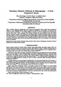
For a plane quadrilateral 2 G with straight edges and vertices P0 , P1 , P2 and P3 (the numbering is counterclockwise) the mapping is bilinear: O D P0 C O1 .P1 P0 / C O2 .P3 P0 / C O1 O2 .P2 P3 C P0 P1 / : (4.15) Figure 4.1 illustrates Definition 4.1.2 for a triangular and a quadrilateral element.

affine

affine affine

Fig. 4.1 Schematic illustration of the reference mappings; triangular panel (left), parallelogram (right)

188


Exercise 4.1.3. Show the following: (a) The affine mapping in (4.14) is regular if and only if P0 , P1 , P2 are vertices of a non-degenerate (plane) triangle , i.e., they are not colinear. Find an estimate for the constants min , max from Definition 4.1.2(b) in terms of the interior angles of . (c) Let P0 ; P1 ; P2 ; P3 be the vertices of a plane quadrilateral with straight edges. The mapping from (4.15) is regular if all interior angles are smaller than and larger than 0. In some cases we will impose a compatibility condition for the intersection of two panels. Definition 4.1.4. A surface mesh G of is called regular if: (a) The intersection of two different elements ; 0 2 G is either empty, a common vertex or a common side. (b) The parametrizations of the panel edges of neighboring panels coincide: For every pair of different elements ; 0 2 G with common edge e D \ 0 we have jeO D 0 ı ; 0 jeO ; where eO WD 1 .e/ and ; 0 W O ! O is a suitable affine bijection. Remark 4.1.5. Throughout this section we assume that the boundary is Lipschitz and admits a regular surface mesh in the sense of Definitions 4.1.2 and 4.1.4. This is a true restriction since not every Lipschitz surface admits a regular surface mesh. For later error estimates we will introduce a few geometric parameters, which represent a measure for the distortion of the panels as well as bounds for their diameters. Assumption 4.1.6. There exist open subsets U; V R3 and a diffeomorphism W U ! V with the following properties: (a) U . (b) For every 2 G, there exists a regular reference mapping W O ! of the form W O ! ; D ı affine W R2 ! R3 is a regular, affine mapping. where affine Example 4.1.7. 1. Let be a piecewise smooth surface that has a bi-Lipschitz continuous paraaffine O O WD metrization over the ˚ affine polyhedral surface : W ! . Let G O i W 1 i N be a regular surface mesh of˚ with the associated ref erence mappings affine W O ! affine . Then G WD affine W affine 2 G affine affine defines a regular surface mesh of which satisfies Assumption 4.1.6.


189

˚ 2. For the unit sphere WD x 2 R3 W kxk D 1 one can choose the inscribed double pyramid with vertices .˙1; 0; 0/| , .0; ˙1; 0/| , .0; 0; ˙1/| as a polyhedral O while W O ! is defined by .x/ WD x= kxk. By means of , surface , regular surface meshes on can then be generated through lifting of regular O surface meshes of the polyhedral surface . In order to construct a sequence of refined surface meshes for , in many cases the procedure is as follows. Remark 4.1.8. Let be the surface of a bounded Lipschitz domain R3 . In the first step we construct a polyhedron O along a bi-Lipschitz continuous mapping W O ! (see Example 4.1.7). Let G0affine be a (very coarse) surface ˚ O Then G0 WD D affine W affine 2 G affine defines a coarse surmesh of . affine 0 of finer surface meshes if, face mesh of . We can obtain a sequence G` ` during each refinement, we decompose every panel in G0affine into new panels by means of a fixed refinement method. For triangular elements, for example, we interconnect the midpoints of the sides and for quadrilateral elements we connect both pairs midpoints. This gives us a sequence of surface meshes by ˚ of opposite G` WD D affine W affine 2 Gàffine . Convention 4.1.9. If and affineappear in the same context the relation between the two is given by D affine . The following definition is illustrated in Fig. 4.2. Definition 4.1.10. Let Assumption 4.1.6 be satisfied. The constants caffine > 0 (Caffine > 0) are the maximal (minimal) constants in caffine kx yk k .x/ .y/k Caffine kx yk 8x; y 2 affine ; 8 affine 2 G affine and describe the distortion of curved panels compared to their affine pullbacks affine . The diameter of a panel 2 G is given by h WD sup kx yk x;y2

and the inner width by the incircle diameter of affine .

Fig. 4.2 Diameter of a panel and incircle diameter; triangular panel (left), parallelogram (right)

190


The mesh width hG of a surface mesh G is given by hG WD maxfh W 2 Gg:

(4.16)

We write h instead of hG if the mesh G is clear from the context. Remark 4.1.11. For plane panels , is the incircle diameter of . The diameters of and affine satisfy 1 h Caffine

sup x;y2 affine

1 h : kx yk D h affine caffine

Definition 4.1.12. The shape-regularity constant G is given by G WD max 2G

h :

(4.17)

For some theorems we will assume, apart from the shape-regularity, that the diameters of all triangles are of the same order of magnitude. Definition 4.1.13. The constant qG that describes the quasi-uniformity is given by qG WD hG = min fh W 2 Gg : Remark 4.1.14. In order to study the convergence of boundary element methods, we will consider sequences .G` /`2N of surface meshes whose mesh width h` WD hG` tends to zero. It is essential that the constant for the shape-regularity ` WD G` remains uniformly bounded above: sup ` < 1:

(4.18)

`2N

In a similar way the constants of quasi-uniformity q` WD qG` have to be bounded above in some theorems: sup q` q < 1: (4.19) `2N

We call a mesh family .G` /`2N with the property (4.18) shape-regular and with the property (4.19) quasi-uniform. Exercise 4.1.15. Show the following: (a) If the surface mesh G0 is regular and if finer surface meshes .G` /` are constructed according to the method described in Remark 4.1.8 then all surface meshes .G` /` are regular. (b) The constants concerning shape-regularity and quasi-uniformity are, under the conditions in Part (a), uniformly bounded with respect to `.


191

4.1.3 Discontinuous Boundary Elements The boundary element method defines an approximation of the unknown density ' in the boundary integral equation (4.6) which is described by finitely many parameters. This can, for example, be achieved by (piecewise) polynomials on the elements of a mesh G. Example 4.1.16. (Piecewise Constant Boundary Elements) Let D @ be piecewise smooth and let G be a – not necessarily regular – surface mesh on . Then SG0 denotes all piecewise constant functions on the mesh G SG0 WD f

2 L1 ./ j 8 2 G W

j is constantg :

(4.20)

Since 2 L1 ./, we only need to define in the interior of an element, as the boundary @, i.e., the set of edges and vertices of the panel, is a set of zero measure. Every function 2 SG0 is defined by its values on the elements 2 G and can be written in the form X (4.21) .x/ D b .x/ 2G

with the characteristic function b W ! R of 2 G: ( 1 x 2 ; b .x/ WD 0 otherwise:

(4.22)

In particular, SG0 is a vector space of dimension N D #f W 2 Gg with basis fb W 2 Gg. In many cases the piecewise constant approximation of the unknown density converges too slowly and, instead, one uses polynomials of degree p 1. In the same way as in Example 4.1.16 this leads to the boundary element spaces SGp . For their definition we need polynomials of total degree p on the reference element as well as the convention for multi-indices from (2.67) ˚ Pp D span W 2 N02 ^ j j p : (4.23) For p D 1 and p D 2, Pp contains all polynomials of the form a00 C a10 1 C a01 2 8a00 ; a10 ; a01 2 R for p D 1; a00 C a10 1 C a01 2 C a20 12 C a11 1 2 C a02 22 8a00 ; a10 ; a01 ; a20 ; a11 ; a02 2 R for p D 2:

Definition 4.1.17. Let D @ be piecewise smooth and let G be a surface mesh of . Then, for p 2 N0 , o n (4.24) SGp WD W ! K j 8 2 G W ı 2 Pp : We simply write S p or only S if the reference to the surface mesh G is obvious.

192


Remark 4.1.18. Note that in (4.24) the functions 2 S p do not constitute polynomials on the surface . Only once they have been “transported back” to the reference element O by means of the element mapping (see Fig. 4.1) is this the case. The parametrizations of the elements 2 G in Definition 4.1.2 (b,c) are thus part of the set SGp . A change in parametrization will lead (with the same mesh G) to a different SGp . Therefore for a mesh G we summarize the element mappings in the mapping vector WD f W 2 Gg

(4.25)

p . and instead of (4.24) we write SG;

Remark 4.1.19. Note that (4.24) also holds for meshes G with quadrilateral elements, i.e., with reference element O D .0; 1/2 . Since S p does not require continuity across element boundaries, the space of polynomials Pp in (4.23) can also be applied to quadrilateral meshes. For the realization of the boundary element spaces we need a basis for Pp , which b .i;j / . O1 ; O2 / and which satisfies we denote by N n o b .i;j / W 0 i; j p; i C j p : Pp D span N

(4.26)

b .i;j / . 1 ; 2 / WD O i O j , 0 i C j p as in (4.23), would be For example, N 1 2 admissible basis functions. Remark 4.1.20. (Nesting of Spaces) We have Pp Pq for all p q. Therefore we can always choose a basis in Pq b .i;j / which contains the basis functions from Pp as a subset. The basis functions N in (4.23) have this property. O on O , every b .i;j / . / Once we have determined a basis N 2 G can be written as X b .i;j / ı 1 ˛i;j N j D

p 2 SG; on a panel

0i Cj p

and

1 b N.i;j / WD N .i;j / ı

spans the restriction f j W suitable indices, we define

0i Cj p

p 2 S p .; G; /g. In order to give a basis of SG;

˚ p WD 2 N02 W j j p : Thus we have

˚ p D span b.;/ .x/ W . ; / 2 p G ; SG;

(4.27)


193

where the global basis functions bI .x/ with the multi-index I D . ; / denote the zero extension of the element function N to : For I D . ; / 2 p G DW I .G; p/ DW I we explicitly have

( bI .x/ WD

Hence, every

(4.28)

N .x/; x 2 ; 0

(4.29)

otherwise:

can be written as a combination of the basis function bI .x/: .x/ D

X I

bI .x/;

x 2 ;

2 G:

(4.30)

I 2I p Let jGj be the number of elements in the mesh G. The dimension of SG; or the number of degrees of freedom is then given by p /: N D jGj .p C 1/.p C 2/=2 D dim.SG; p is then uniquely characterized by the vector . Every function in 2SG; N I.G;p/ R ŠR as in (4.30).

(4.31) I /I 2I.G;p/

4.1.4 Galerkin Boundary Element Method The simplest boundary element method for Problem (4.6) consists in approximating the unknown density ' in (4.9) by a piecewise constant function 'S 2 S 0 .; G/. Convention 4.1.21. The boundary element functions depend on the boundary element space S p .; G; /; in particular, they depend on , the surface mesh G and the polynomial degree p. We will, whenever possible, use the abbreviated notation 'S instead of 'SGp; . Inserting (4.30) into (4.6) or into the variational formulation (4.8) leads to a contradiction: since, in general, we have 'S 6D ', (4.6) and (4.8) cannot be satisfied with ' D 'S , which is why the statements have to be weakened. As 'S is determined by N parameters 'IS I 2I [see (4.29)–(4.31)], we are looking for N conditions to determine 'IS . In the Galerkin boundary element method we only let the test function run through a basis of SGp in the variational formulation of the boundary integral equation (4.9). The Galerkin approximation of the integral equation (4.9) then reads:

194


p Find 'S 2 SG; such that

b.'S ; S / D F .S /

p

8S 2 SG; ;

(4.32)

with b.; / and F ./ from (4.10) and (4.11) respectively. Remark 4.1.22. (i) The Galerkin discretization (4.32) of (4.8) is achieved by resp tricting the trial and test functions '; to the subspace SG; H 1=2 ./ in the variational formulation (4.8). (ii) The boundary element solution 'S in (4.32) is independent of the basis chosen for the subspace. The computation of the approximation 'S requires that we choose a concrete basis for the subspace. Therefore, [see (4.29)–(4.31)] for a fixed p 2 N0 , we choose the basis (4.33) .bI W I 2 I .G; p// p

for SG; . Then (4.32) is equivalent to the linear system of equations: Find ' 2 RN such that B ' D F:

(4.34)

Here the system matrix B D .BI;J /I;J 2I.G;p/ and the right-hand side F D .FJ /J 2I.G;p/ 2 RN with I D . ; / and J D .; t/ are given by BI;J WD b.bI ; bJ / Z Z Z Z Nt .x/ N .y/ bJ .x/ bI .y/ dsy dsx D dsy dsx D 4 kx yk t 4 kx yk Z Z FJ WD F .bJ / D gD .x/bJ .x/ dsx D gD .x/Nt .x/ dsx :

(4.35)

(4.36)

t

Remark 4.1.23. The matrix B in (4.34) is dense because of (4.35), which means that all entries BI;J are, in general, not equal to zero. Furthermore, the twofold surface integral in (4.35) can very often not be computed exactly, even for polyhedrons, and requires numerical integration methods for its approximation. The influence of this additional approximation will be discussed in Chap. 5. In this chapter we will always assume that the matrix B can be determined exactly. Proposition 4.1.24. The system matrix B in (4.34) is symmetric and positive definite. Proof. From the symmetry of b.'; / D b.; '/ we immediately have BI;J D b.bI ; bJ / D b.bJ ; bI / D BJ;I ; and subsequently B D B| . Now let ' 2 RN be arbitrary. Then we have

4.1 Boundary Elements for the Potential Equation in R3 |

' B' D

X

'J 'I BI;J D

I;J 2I.G;p/

X

195

'J 'I b.bI ; bJ / D b

I;J

X

' I bI ;

I

X

! ' J bJ

J

D b.'S ; 'S / k'S k2H 1=2 ./ > 0 if and only if 'S 6D 0. Since fbI W I 2 Ig is a basis of S p , we have 'S 6D 0 if and only if ' 6D 0 2 RN . Therefore B is positive definite. p

Thus the discrete problem (4.32) or (4.34) has a unique solution 'S 2 SG . The following proposition supplies us with an estimate for the error ' 'S . Proposition 4.1.25. Let ' be the exact solution of (4.9). The Galerkin solution 'S of (4.32) converges quasi-optimally k' 'S kH 1=2 ./

kbk min k' S kH 1=2 ./ : S 2S p

(4.37)

The error satisfies the Galerkin orthogonality b.' 'S ; S / D 0

8S 2 S p :

(4.38)

Proof. We will first prove the statement in (4.38). If we only consider (4.10) for test functions from S p we can subtract (4.32) and obtain b.' 'S ; S / D b.'; S / b.'S ; S / D F .S / F .S / D 0

8S 2 S p :

Next we prove (4.37). For the error eS D ' 'S we have by the ellipticity and the continuity of the boundary integral operator V and (4.38) k' 'S k2H 1=2 ./ b.eS ; eS / D b.eS ; ' 'S / D b.eS ; '/ b.eS ; 'S / D b.eS ; '/ b.eS ; S / D b.eS ; ' S / kbkkeS kH 1=2 ./ k' S kH 1=2 ./

for all S 2 S p . If we cancel keS kH 1=2 ./ and minimize over S 2 S p we obtain the assertion (4.37). The inequality in (4.37) shows that the Galerkin error k' 'S kH 1=2 ./ coincides with the error of the best approximation of ' in S p up to a multiplicative constant. This is where the term quasi-optimality for the a priori error estimate (4.37) originates. Remark 4.1.26 (Collocation). We obtained the Galerkin discretization (4.32) from (4.8) by restricting the trial and test functions '; to the subspace S p S . Alternatively, one can insert 'S into (4.6) and impose the equation

196


.V 'S /.xJ / D gD .xJ /

J 2 I .G; p/

(4.39)

only in N collocation points fxJ W J 2 Ig. The solvability of (4.39) depends strongly on the choice of collocation points fxJ W J 2 Ig. Equation (4.39) is also equivalent to a linear system of equations, where the entries of the system matrix Bcol l are defined by Z bJ .y/ col l dsy : (4.40) BI;J WD 4 kxI yk Note that Bcol l is again dense, but not symmetric. The collocation method (4.39) is widespread in the field of engineering, because the computation of the matrix entries (4.40) only requires the evaluation of one integral over the surface , instead of, as with the Galerkin method, a twofold integration over . However, the stability and convergence of collocation methods on polyhedral surfaces is still an open question, especially with integral equations of the first kind. For integral operators of zero order or equations of the second kind we only have stability results in some special cases. For a detailed discussion on collocation methods we refer to, e.g., [6, 8, 87, 187, 207, 215] and the references contained therein. We now return to the Galerkin method. Remark 4.1.27 (Stability of the Galerkin Projection). The (4.32) defines a mapping p W …pS W H 1=2 ./ ! SG;

Galerkin

method

…pS ' WD 'S ; p

which is called the Galerkin projection. Clearly, …S is linear and because of the ellipticity of the boundary integral operator V we have k…pS 'k2H 1=2 ./ D k'S k2H 1=2 ./ b.'S ; 'S / D b.'; 'S / kbkk'kH 1=2 ./ k…pS 'kH 1=2 ./ ; from which we have, after canceling, the boundedness of the Galerkin projection 1 1 p …S W H 2 ./ ! H 2 ./ independent of the mesh G: k…pS 'kH 1=2 ./

kbk k'kH 1=2 ./ :

(4.41)

The quasi-optimality (4.37) and the boundedness of the Galerkin projection combined with the following corollary give us the convergence of the Galerkin BEM. Corollary 4.1.28. Let .G` /`2N be a sequence of meshes on with a mesh width h` D hG` and let h` ! 0 for ` ! 1. Then the sequence .'` /`2N of boundary element solutions (4.32) in S` D SGp` converges to ' for every fixed p 2 N0 .


197

Proof. Since S`0 S`p for all p 2 N0 , we will only consider the case p D 0. S`0 are step functions on meshes whose mesh width converges to zero. The density follows from the construction of the Lebesgue spaces [ `2N

S`0

kkL2 ./

D L2 ./

and from Proposition 2.5.2 we have the dense embedding L2 ./ H 1=2 ./. For ' 2 H 1=2 ./ and an arbitrary " > 0 we can therefore choose a 'Q from 2 L ./ and an ` 2 N, combined so that 'Q` 2 S`0 , such that Q H 1=2 ./ "=2 and k' 'k

k'Q 'Q` kL2 ./ "=2:

From this we have Q H 1=2 ./ C k'Q 'Q` kH 1=2 ./ k' 'Q` kH 1=2 ./ k' 'k

" " C ": 2 2

The quasi-optimality of the Galerkin method gives us k' '` kH 1=2 ./

kbk kbk : k' 'Q` kH 1=2 ./ "

As " > 0 is arbitrary, we have the assertion for ` ! 1.

4.1.5 Convergence Rate of Discontinuous Boundary Elements We have seen in Proposition 4.1.25 that the approximations 'S 2 S from the Galerkin boundary element method approximate the exact solution ' of the equation of the first kind (4.9) quasi-optimally: the error ' 'S , which is measured in the “natural” H 1=2 ./-norm, is – up to a multiplicative constant – just as large as ˚ min k'

S kH 1=2 ./

W

S

2S

(4.42)

which is the error of the best approximation in the space S . The convergence rate of the BEM indicates how fast the error converges to zero in relation to an increase in the degrees of freedom N . Here we will only prove the convergence rate for p D 0, while the general case will be treated in Sect. 4.3. We begin with the second Poincaré inequality on the reference element . O Convention 4.1.29. Variables on the reference element are always marked by a “ˆ”. If the variables x 2 and xO 2 O appear in the same context this should always be understood in terms of the relation x D .Ox/. Derivatives with respect to variables in the reference element are also marked by a “ˆ”. We will write, for b as an abbreviation for rxO . Should the functions u W ! K and uO W O ! example, r K appear in the same context, they are connected by the relation u ı D uO .

198


Proposition 4.1.30. Let O R2 be the reference element, 'O 2 H 1 .O / and 'O0 WD R 1 'O d xO . Then there exists some cO > 0 such that jO j O b'k k'O 'O0 kL2 ./ O r O L2 ./ O ck O ;

(4.43)

where cO depends only on O . Proof. The assertion follows directly from the proof of Corollary 2.5.10.

In the following we will derive error estimates for a simplified situation. We will discuss the general case in Sect. 4.3. Here we let be a plane manifold in R3 with a polygonal boundary. As integrals are invariant under rotation and translation, we assume without loss of generality that is a two-dimensional polygonal domain,

(4.44)

i.e., we restrict ourselves to the two-dimensional approximation problem in the plane. Furthermore, let G D fi W 1 i N g be a surface mesh on of shape-regular triangles with straight edges and with mesh width h > 0. Then the triangles 2 G are affinely equivalent to the reference element O via the transformation (4.14): 3 x D .Ox/ D P0 C JOx;

xO 2 ; O

(4.45)

where J is the matrix with the columns P1 P0 and P2 P1 (see Fig. 4.1). With (4.45) and the chain rule @ @xO 1 @ @xO 2 @ D C @x˛ @xO 1 @x˛ @xO 2 @x˛ the relation

| b r D J1 r;

˛ D 1; 2;

d x D .det J/ d xO D 2 jj d xO

follows. This leads to the transformation formula for Sobolev norms Z Z jj O 2 2 b b D jr 'j O d xO D .r'/> JJ> .r'/d x kr 'k O L2 ./ O jj O Z jj O kr'k2 d x; jj

(4.46)

(4.47)

where denotes the largest eigenvalue of JJ| 2 R22 . Furthermore, we have for the left-hand side of (4.43) k'O 'O0 k2L2 ./ D O

jj O k' '0 k2L2 ./ jj

(4.48)


with '0 WD

1 jj

R

199

'd x. If we combine (4.48) with (4.43) and (4.47) we obtain jj jj r 'k O 2L2 .O / cO 2 kr'k2L2 . / 8 2 G : k'O 'O0 k2L2 .O / cO 2 kb O O jj jj (4.49)

k' '0 k2L2 . / D

Exercise 4.1.32 shows that kP1 P0 k2 C kP2 P1 k2 2h2 : From this we have k' '0 kL2 ./

p

(4.50)

2ch O j'jH 1 ./ :

(4.51)

Squaring and then summing over all 2 G leads to the following error estimate. Proposition 4.1.31. Let (4.44) hold. Let G be a surface mesh of . Let ' 2 L2 ./ with 'j 2 H 1 ./ for all 2 G. Then we have the error estimate min k' 0 2SG

kL2 ./

X p 2cO h2 j'j2H 1 ./

!1=2 :

(4.52)

2G

For ' 2 H 1 ./ the error estimate can be simplified to min k' kL2 ./ 0 2SG

p 2ch O G j'jH 1 ./ :

(4.53)

Exercise 4.1.32. Let be a plane triangle with straight edges in R2 with vertices P0 , P1 , P2 . Let the matrix J and the eigenvalue be defined as in (4.45) and (4.47) respectively. Show that kP1 P0 k2 C kP2 P1 k2 : From the approximation property we will now derive an error estimate for the Galerkin solution. Theorem 4.1.33. Let be the surface of a polyhedron. Let the surface mesh G consist of triangles with straight edges. For the solution ' of the integral equation of the first kind (4.6) we assume that for an 0 s 1 we have (4.54) ' 2 H s ./: Then the Galerkin approximation 'S 2 SG0 satisfies the error estimate k' 'S kH 1=2 ./ C hsC1=2 k'kH s ./ :

(4.55)

Proof. The conditions of the theorem allow us to apply Proposition 4.1.31. With (4.37) we obtain for the Galerkin solution 'S the error estimate

200


k' 'S kH 1=2 ./ D k' …0S 'kH 1=2 ./

kbk min k' S 2SG0

S kH 1=2 ./ :

The definition of the H 1=2 ./-norm gives us k'

S kH 1=2 ./

D

.'

sup

S ; /L2 ./

kkH 1=2 ./

2H 1=2 ./nf0g

:

(4.56)

We will first consider the case ' 2 H 1 ./ and choose S elementwise as the mean value of ' Z 1 WD ' d x; 2 G; P ' WD S with j S jj i.e., P is the L2 -orthogonal projection onto SG0 . Hence it follows from Proposition 4.1.31 that k

S kL2 ./ k'kL2 ./ ;

k'

S kL2 ./

2k'kL2 ./ ; k'

S kL2 ./

chk'kH 1 ./ : (4.57)

If in Proposition 2.1.62 we choose T D I P we have T W L2 ./ ! L2 ./ and T W H 1 ./ ! L2 ./. For the norms we have, by (4.57), the estimates kT kL2 ./

L2 ./

2

and

kT kL2 ./

H 1 ./

ch:

Proposition 2.1.62 implies that T W H s ./ ! L2 ./ for all 0 s 1 and that kT kL2 ./

H s ./

chs :

This is equivalent to the error estimate k'

S kL2 ./

c hs k'kH s ./ :

(4.58)

In order to derive an error estimate for the H 1=2 ./-norm, we use (4.56) and note that the equality j .'

S ; /L2 ./

j D j .'

S;

S /L2 ./ j

holds for an arbitrary S 2 SG0 . By using ' 2 H s ./, 2 H 1=2 ./ and (4.58) and by choosing S elementwise as the integral mean value of , we obtain the estimate ˇ ˇ.'

S ; /L2 ./

ˇ ˇ ˇ D ˇ.'

S;

ˇ S /L2 ./ ˇ k'

ch k'kH s ./ h s

1=2

kkH 1=2 ./ :

S kL2 ./ k

S kL2 ./


201

The error estimate (4.55) shows that the convergence rate hsC1=2 of the BEM depends on the regularity of the solution '. In Sect. 3.2 we stated the regularity – the maximal s > 0 such that ' 2 H 1=2Cs ./ – without knowing the exact solution ' explicitly. Ideally, ' is smooth on the entire surface .s D 1) or at least on every panel. The convergence rate would then be bounded by the polynomial order p of the boundary elements, due to the fact that the following generalization of Theorem 4.1.33 holds. Corollary 4.1.34. Let the exact solution of (4.9) satisfy ' 2 H s ./ for an s 0. p Then the boundary element solution 'S 2 SG satisfies the error estimate 1=2Cmin.s;pC1/

k' 'S kH 1=2 ./ chG

k'kH s ./ ;

(4.59)

for a surface mesh G of the boundary , which consists of triangles with straight edges. Here the constant c depends on p and the shape-regularity of the surface mesh. The proof of Corollary 4.1.34 will be completed in Sect. 4.3.4 (see Remark 4.3.21).

4.1.6 Model Problem 2: Neumann Problem Let R3 be a bounded interior domain with boundary and C WD R3 n . For gN 2 H 1=2 ./ we consider the Neumann problem u D 0 1 u D gN 1

ju .x/j C kxk

in C ;

(4.60)

on ;

(4.61)

for kxk ! 1:

(4.62)

The exterior problem (4.60)–(4.62) has a unique solution u, which can be represented as a double layer potential 1 u.x/ D 4

Z '.y/

1 @ dsy ; @ny kx yk

x 2 C :

Thanks to the jump relations (see Corollary 3.3.12)

1 4

Z

8 ˆ ˆ 1 x 2 ; < @ 1 1 dsy D 2 x 2 and is smooth in x ˆ @ny kx yk ˆ : 0 x 2 C

(4.63)

202


u.x/ in (4.63) does not change if a constant is added to '. If we put (4.63) into the boundary condition (4.61) we obtain the equation W' D

@ @nx

1 4

Z '.y/

@ 1 dsy @ny kx yk

D gN .x/;

x 2 :

(4.64)

The following remark shows that the derivative @=@nx and the integral do not commute. Remark 4.1.35. The normal derivative @=@nx , applied to the kernel in (4.64), yields ˝ ˝ ˛ ˛ nx ; ny hnx ; x yi ny ; x y 1 @2 3 : D @nx @ny kx yk kx yk3 kx yk5 Therefore the kernel of the associated hypersingular integral operator is not integrable. There are three possibilities of representing the integral operator W ' on the surface: (a) by extending the definition of an integral to strongly singular kernel functions (see [201, 211]), (b) by integration by parts (see Sect. 3.3.4) and (c) by introducing suitable differences of test and trial functions (see [117, Sect. 8.3]). In this section we will consider option (b). The notation and theorems from Sect. 3.3.4 can be simplified for the Laplace problem, so that they read curl ' WD 0 .grad Z '/ n; Z Z hcurl ' .y/; curl .x/i b.'; / D dsy dsx ; 4 kx yk where Z W H 1=2 ./ ! H 1 . / is an arbitrary extension operator (see Theorem 2.6.11 and Exercise 3.3.25). The variational formulation of the boundary integral equation is given by (see Theorem 3.3.22): Find ' 2 H 1=2 ./=K such that b.'; / D .gN ; /L2 ./

8 2 H 1=2 ./=K:

(4.65)

In Theorem 3.5.3 we have already shown that the density ' in (4.63) is the unique solution of the boundary integral equation (4.65). The proof was based on the fact that the bilinear form b .; / is symmetric, continuous and H 1=2 ./ =K-elliptic.

4.1.7 Continuous Boundary Elements The Galerkin method is based on the concept of replacing the infinite-dimensional Hilbert space by a finite-dimensional subspace. The bilinear form that is associated with the hypersingular integral operator is defined on the Sobolev space


203

H 1=2 ./ =K. As the discontinuous boundary element functions from Example 4.1.16 and Definition 4.1.17 are not contained in H 1=2 ./ =K (see Exercise 2.4.4), we will introduce continuous boundary element spaces for the Neumann problem. We again start with a mesh G on the boundary . In order to define continuous boundary elements, we assume (see Definition 4.1.4): The surface mesh G is regular.

(4.66)

This means that the intersection \ 0 of two different panels is either empty, a vertex or an entire edge. Furthermore, the boundary elements are either triangles or quadrilaterals and are images of the reference triangle or quadrilateral O respectively (see Fig. 4.1). Note that the boundary edges of the panels “have the same parametrization on both sides” in the case of continuous boundary elements (see Definition 4.1.4). We assume that the boundary is piecewise smooth (see Definition 2.2.10 and Fig. 4.1) so that the reference mappings W O ! can be chosen as smooth diffeomorphisms. As in the case for discontinuous boundary elements, the continuous boundary elements are also piecewise polynomials on the surface . When using discontinuous elements, a boundary element function 'S is locally a polynomial of degree p in each element 2 G: 8 2 GW

O 'S ı 2 Pp ./:

With continuous elements we have for 2 G: 8 < Pp if is a triangular element, 'S ı 2 Pp WD : P if is a quadrilateral element, p

(4.67)

where for p 1 the polynomial space Pp is defined as in (4.23) and Pp WD spanf O1i O2j W 0 i; j pg: Now we come to the definition of continuous boundary element functions of degree p 1. Definition 4.1.36. Let be a piecewise smooth surface, G a regular surface mesh of and D f W 2 Gg the mapping vector. Then the space of continuous boundary elements of degree p 1 is given by p;0 WD f' 2 C 0 ./ j 8 2 G W 'j ı 2 Pp g: SG;

In order to make the distinction between continuous and discontinuous boundary p;1 . elements of degree p we will from now on denote discontinuous elements by SG;

204


Just like the space S p;1 of discontinuous boundary elements, the space S p;0 is also finite-dimensional. In the following we will introduce a basis f'I W I 2 Ig of S p;0 . In contrast to S p;1 , the support of the basis functions in general consists of more than one panel and the basis functions are defined piecewise on those panels. We begin with the simplest case, p D 1. Example 4.1.37. (Linear and Bilinear, Continuous Boundary Elements) b .Ox/, xO D .xO 1 ; xO 2 / on the reference element O are: The shape functions N |

|

In the case of the unit triangle with vertices P0 D .0; 0/ , P1 D .1; 0/ , P2 D |

.1; 1/ [see (4.13)], given by b 0 .Ox/ D 1 xO 1 ; N

(4.68)

b 1 .Ox/ D xO 1 xO 2 ; N b 2 .Ox/ D xO 2 N and

|

|

In the case of the unit square with vertices P0 D .0; 0/ , P1 D .1; 0/ , P2 D |

|

.1; 1/ , P3 D .0; 1/ , given by

b 0 .Ox/ D .1 xO 1 /.1 xO 2 /; N

(4.69)

b 1 .Ox/ D xO 1 .1 xO 2 /; N b 2 .Ox/ D .1 xO 1 / xO 2 ; N b 3 .Ox/ D xO 1 xO 2 : N b i is equal to 1 at the vertex Pi of the reference We notice that the shape function N element 1 and vanishes at all other vertices (see Fig. 4.3). b i W i D 0; 1; 2g and P .b b O D spanfN It holds P1 ./ 1 / D spanfN i W i D 0; : : : 3g. For the definition of the boundary element spaces of polynomial degree p we have to distinguish between quadrilateral elements and triangular elements. For the reference element O 2 G and p 2 N0 we define the index set

2

Fig. 4.3 Reference elements O D S2 (left) and O D Q2 (right) and nodal points for P1O

2

1

1


205

.2/ Fig. 4.4 Nodal points PO i;j for the reference triangle (left) and for the unit square (right)

1,2 1,1

2,1

0,1

1,0

pO

1,1

2,1

1,0

˚ .i; j / 2 N02 W 0 j i p in the case of the unit triangle, ˚ WD .i; j / 2 N02 W 0 i; j p in the case of the unit square.

(4.70)

We will omit the index O in pO if the reference element is clear from the context. Example 4.1.38 (Boundary elements of degree p > 1). The trial spaces Pp , Pp b .p/ 2 PpO which will be defined next. The in (4.67) are spanned by the functions N .i;j /

nodal points for the reference element O are given by b .p/ P .i;j / WD

i j ; p p

| ;

8 .i; j / 2 pO

(4.71)

(see Fig. 4.4). b .p/ is characterized by For .i; j / 2 pO the shape function N .i;j / b .p/ 2 PpO N .i;j /

b .p/ .P b .p/ and N .k;`/ / D .i;j /

1 .k; `/ D .i; j / ; 0 .k; `/ 2 pO n f.i; j /g

(see Theorem 4.1.39). Theorem 4.1.39. Let k 2 N. Then every q 2 PkO is uniquely determined by its o n values in †k WD .i=k; j=k/ W .i; j / 2 kO . The set †k is called unisolvent for the polynomial space PkO because of this property. Proof. A simple calculation shows that dim PkO D ]†k : Therefore it suffices to prove either one of the following statements (a) or (b): (a) For every vector .bz /z2†k there exists a q 2 PkO such that q .z/ D bz for all z 2 †k : (b) If q 2 PkO and q .z/ D 0 for all z 2 †k then q 0.

206


b by Case 1: O D .0; 1/2 : For 2 kO we define the function N Q Qk kxj ij b .x/ WD 2 N : ij D0 j D1 ij ¤j j ij b 2 P O with N b . =k/ D 1 and N b i1 ; i2 D 0 for all .i1 ; i2 / 2 O n f g. Then N k k k k Now let b 2 O be arbitrary. Then the polynomial q 2 PkO k

q .x/ D

X

b .x/ b N

O 2 p

satisfies property (a). Case 2: O is the reference triangle. As in Example 4.1.37 we set O 1 .x/ WD 1 xO 1 ;

O 2 .x/ WD xO 1 xO 2 ;

O 3 .x/ WD xO 2 :

Clearly, these functions are in P1O and have the Lagrange property 81 i; j 3 W O i Aj D ıi;j with A1 D .0; 0/| , A2 D .1; 0/| , A3 D .1; 1/| : 1. k D 1W For a given .bi /3iD1 2 R3 , q 2 P1 W q .x/ D

3 X

bi O i .x/

i D1

clearly has the property (a). 2. k D 2W For 1 i < j 3, A.i;j / WD Ai C Aj =2 denote the midpoints of the edges of O . We define b i WD O i 2O i 1 1 i 3; N b .i;j / WD 4O i j N 1 i < j 3: b .i;j / 2 P O and bk, N Then we clearly have N 2 b i Aj D ıi;j N b i A.k;`/ D 0 N 8i; k; `; b .i;j / .Ak / D 0 N b .i;j / A.k;`/ D ıi;k ıj;` 8i; j; k; `: N ˚ For a given fbz W z 2 †2 g D bi ; b.k;`/ , the polynomial q 2 P2O defined by q .x/ WD

3 X i D1

has the property (a).

b i .x/ C bi N

X 1k 1. t t ./ with t > 1. Let TGp W Hpw ./ ! SGp;0 be defined by Now let ' 2 Hpw TGp

WD

QG if t D 1; IGp if t > 1:

Proposition 4.1.50 implies that TGp is continuous. The estimate k' 'S kH 1=2 ./=K

kbk kbk k' TGp 'kH 1=2 ./=K k' TGp 'kH 1=2 ./

follows from the quasi-optimality (4.84), and we have used k'kH 1=2 ./=K D min k' ckH 1=2 ./ k'kH 1=2 ./ . c2R

If we apply Proposition 2.1.65 with X0 D L2 ./, X1 D H 1 ./ and D 1=2 we obtain the interpolation inequality k'k2H 1=2 ./ k'kL2 ./ k'kH 1 ./ : With this and with Proposition 4.1.50 it follows for t 1 that

218


k' TGp 'k2H 1=2 ./ C k' TGp 'kL2 ./ k' TGp 'kH 1 ./ C h2 min.t;pC1/1 k'k2H t

(4.95)

pw ./

and therefore we have (4.94) for t > 1. Case 3: 1=2 < t 1: In this case we prove (4.94) by interpolation. We have for the operator I QG the estimate [cf. Proposition 4.1.50(b)] kI QG kH 1=2 ./

H 1=2 ./

C;

kI QG kH 1=2 ./

H 1 ./

C h1=2 :

As in the proof of Theorem 4.1.33, the estimate 1

k.I QG /'kH 1=2 ./ C ht 2 k'kH t ./ : follows for 1=2 t 1 by interpolation of the linear operator I QG : H t ./ ! 1 H 2 ./ (see Proposition 2.1.62).

4.1.10 Model Problem 3: Mixed Boundary Value Problem We consider the mixed boundary value problem for the Laplace operator: u D 0

in ,

u D gD

on D ,

@u=@n D gN

on N

(4.96)

for given boundary data gD 2 H 1=2 .D /, gN 2 H 1=2 .2 /. For the associated variational formulation we refer to Sect. 2.9.2.3. The approach that allows the discretization of mixed boundary value problems by means of the Galerkin boundary element method is due to [220, 239]. For the treatment of problems with more general transmission conditions we refer to [233]. The problem can be reduced to an integral equation for the pair of densities e 1=2 .N /. The solution of (4.96) can be represented e 1=2 .D / H .'; / 2 H D H with the help of Green’s representation formula u .x/ D .S/.x/ .D'/.x/;

x 2 :

The variational formulation of the boundary integral equation reads [see (3.89)]: Find .'; / 2 H such that bmixed

! !! ' ; D .gD ; /L2 .D / C .gN ; /L2 .N /

8 .; / 2 H (4.97)

This section should be read as a complement to the core material of this book.


219

with bmixed

! !! 0 ' '; L2 . / ; D .VDD '; /L2 .D / .KDN ; /L2 .D / C KND N C .WNN ; /L2 .N / :

The boundary element discretization is achieved by a combination of different boundary element spaces on the pieces D ; N . For this let GD , GN be surface meshes of D ; N , while we assume that GN is regular (see Definition 4.1.4). We use discontinuous boundary elements of order p1 0 on D . The inclusion p ;1

SGD1

e 1=2 .D /; H

(4.98)

results, because the zero extension ? of every function 2 SGpD1 ;1 satisfies the e 1=2 .D /. inclusion ? 2 L2 ./ H 1=2 ./ and thus we have 2 H 1=2 e .N / we define for p2 1 For the approximation of 2 H n o p ;0 p ;0 SGN2 ;0 D 2 SGN2 W j@N D 0

(4.99)

and therefore the boundary values of the functions 2 SGpN2 ;0;0 vanish on @N . satisfies ? 2 Remark 4.1.52. The zero extension ? of functions 2 SGp;0 N ;0 p;0 SG H 1=2 ./, where we have set G WD GD [ GN . With these spaces we can finally formulate the boundary element discretization of (4.97). In the following we will summarize the polynomial orders p1 0 and p2 1 in the vector p D .p1 ; p2 /. Find .'S ; S / 2 S p WD SGpD1 ;1 SGpN2 ;0;0 such that bmixed

'S S

S ; D .gD ; S /L2 .D / C.gN ; S /L2 .N / S

8.S ; S / 2 S p :

(4.100) The norm for functions .'; / 2 H is given by k.'; /kH WD k'kHQ 1=2 .D / C kkHQ 1=2 .N / . Once more the unique solvability of the boundary element discretization of the integral equation follows from the H-ellipticity (3.112) of the bilinear form bmixed , and from the Galerkin orthogonality of the error, we have the quasi-optimality. Theorem 4.1.53. Let .'; / 2 H be the exact solution of (4.97). The discretization (4.100) has a unique solution .'S ; S / 2 S p , p D .p1 ; p2 /, which converges quasioptimally: k.'; / .'S ; S /kH C1 min p k.'; / .; /kH : . ; /2S

(4.101a)

220


s t If the exact solution satisfies .'; / 2 Hpw .D / Hpw .N / for s; t 0 we have the quantitative estimate

1 s . / k.'; / .'S ; S /kH C2 hminfs;p1 C1gC 2 k'kHpw D 1 C hminft;p2 C1g 2 kkHpw t . / : N

(4.101b)

Here the constant C2 depends only on C1 in (4.101a), the shape-regularity (see Definition 4.1.12) of the surface meshes GD , GN and the polynomial degrees p1 and p2 . Proof. For the proof we only need to show the approximation property on the boundary pieces D and N . Here we use (4.59) on D and (4.93) on N for a sufficiently large t > 1. Hence the interpolation IGp ' in (4.93) is well defined and we have p ˇˇ 'j@N D IG ' @ D 0. Therefore the zero extension of the difference function N? satisfies ' IGp ' 2 H 1=2 ./ and from (4.93) with s D 0; 1 we have: p ? p t . / ; k ' IG ' kL2 ./ D k' IG 'kL2 .N / C hmin.t;pC1/ k'kHpw N p ? p k ' IG ' kH 1 ./ D k' IG 'kH 1 .N / C hmin.t;pC1/1 k'kHpw t . / : N (4.102) Then, by interpolation as in the proof of Theorem 4.1.51 and by the boundedness of the Galerkin projection (see Remark 4.1.27), (4.101b) follows.

4.1.11 Model Problem 4: Screen Problems In this section we will discuss the Galerkin boundary element method for the screen problem from Sect. 3.5.3, which is due to [219]. Hence we again assume that an open manifold 0 is given, which can be extended to a closed Lipschitz surface in R3 in such a way that we have for 0c D n 0 D 0 [ 0c : In order to avoid technical difficulties, we require that 0 and 0c be simply connected. We have already introduced the integral equations for the Dirichlet and Neumann screen problems in Sect. 3.5.3: e 1=2 .0 / such Dirichlet Screen Problem: For a given gD 2 H 1=2 .0 / find ' 2 H that e 1=2 .0 /: .V '; /L2 .0 / D .gD ; /L2 .0 / 8 2 H (4.103)



221

e 1=2 .0 / such Neumann Screen Problem: For a given gN 2 H 1=2 .0 / find 2 H that e 1=2 .0 /: 8 2 H (4.104) .W ; /L2 .0 / D .gN ; /L2 .0 / The Galerkin BEM for (4.103) and (4.104) are based on a regular mesh G of 0 and a boundary element space of polynomial degree p1 0 for the Dirichlet problem (4.103) and p2 1 for the Neumann problem (4.104). p ;1 Dirichlet Screen Problem: For a given gD 2 H 1=2 .0 / find 'S 2 SG 1 such that .V

S ; S /L2 .0 /

8S 2 SGp1 ;1 :

D .gD ; S /L2 .0 /

(4.105)

p2 ;0 Neumann Screen Problem: For a given gN 2 H 1=2 .0 / find S 2 SG;0 such that p2 ;0 8 2 SG;0 :

.W S ; S /L2 .0 / D .g; /L2 .0 /

(4.106)

Note that in S0p2 ;0 the boundary data of S on @0 is set to zero (see Remark 4.1.52). With the ellipticity from Theorem 3.5.9 we immediately have the quasi-optimality of the discretization. Theorem 4.1.54. Equations (3.116), (3.117) as well as (4.105), (4.106) have a unique solution and the Galerkin solutions converge quasi-optimally: k

S kH Q 1=2 .0 /

C

min

p ;1

S 2SG 1

k S kHQ 1=2 .0 / C

min

p ;0

2

S 2SG;0

k

S kHQ 1=2 .0 / ;

k S kHQ 1=2 .0 / :

(4.107a)

(4.107b)

s If the exact solution of the Dirichlet problem (3.116) is contained in Hpw .0 / for an s 0 we have

k

Sk Q1 H 2 .0 /

1

s . / : C1 hmin.s;p1 C1/C 2 k kHpw 0

(4.108a)

t .0 / for a t > 1=2 If the exact solution of the Neumann problem is contained in Hpw we have 1

t . / : k S kHQ 1=2 .0 / C2 hmin.t;p2 C1/ 2 kkHpw 0

(4.108b)

Here the constants C1 ; C2 depend only on the respective constant C in (4.107), the shape-regularity (see Definition 4.1.12) of the mesh and the polynomial degrees p1 and p2 . Remark 4.1.55. In general, the exact solutions of the screen problems have edge singularities and therefore they do not have a very high order of regularity s or t in (4.108). Therefore the convergence rates of the Galerkin solutions in (4.108)

222


are low, even for higher order discretizations. This problem can be overcome by an anisotropic mesh refinement near @0 . For details we refer to [221].

4.2 Convergence of Abstract Galerkin Methods All boundary integral operators in Chap. 4.1 were elliptic, which allowed the use of the Lax–Milgram lemma to prove existence and uniqueness. As we have already seen with the Helmholtz problem, however, in certain practical cases we encounter indefinite boundary integral operators. Here we will show for very general subspaces and especially for non-symmetric and non-elliptic sesquilinear forms, under which circumstances the Galerkin solution uS 2 S exists and the error converges quasioptimally. An early study on this subject can be found in [223]. For a study on the convergence of general boundary element methods we refer to [215].

4.2.1 Abstract Variational Problem We would first like to recall the abstract framework from Sect. 2.1.6 and, again, refer, e.g., to [9, Chap. 5], [151, 166, 174] as standard references and additional material. Let H1 ; H2 be Hilbert spaces and a.; / W H1 H2 ! C a continuous sesquilinear form: kak D

ja.u; v/j < 1; u2H1 nf0g v2H2 nf0g kukH1 kvkH2 sup

sup

(4.109)

and let the (continuous) inf–sup conditions hold: There exists a constant > 0 such that ja.u; v/j sup > 0; (4.110a) inf u2H1 nf0g v2H2 nf0g kukH1 kvkH2 and we have 8v 2 H2 n f0g W sup ja.u; v/j > 0:

(4.110b)

u2H1

Then for every functional F 2 H20 the problem Find u 2 H1 W

a.u; v/ D F .v/

8v 2 H2

(4.111)

has a unique solution, which satisfies kukH1

1 kF kH20 :

(4.112)

4.2 Convergence of Abstract Galerkin Methods

223

4.2.2 Galerkin Approximation We require the following construction of approximating subspaces for the definition of the Galerkin method, which we use to solve (4.111). For i D 1; 2, let Sì `2N be given sequences of finite-dimensional, nested subspaces of Hi whose union is dense in Hi i 8` 0 W Sì S`C1 ;

dim Sì < 1

and

[ `2N

Sì

kkHi

D Hi ;

i D 1; 2 (4.113)

and whose respective dimensions satisfy the conditions N` WD dimS`1 D dim S`2 < 1; 8` 2 N W N` < N`C1 ; N` ! 1 for ` ! 1:

(4.114)

Since the dimensions of S`1 and S`2 are equal, it follows that the system matrix for the boundary element method is square. The density implies the approximation property lim minfkui vkHi W v 2 Sì g D 0:

8ui 2 Hi W

`!1

(4.115)

Every ui in Hi can thus be approximated by a sequence vi` 2 Sì . In Sect. 4.1 we p;0 p;1 have already encountered the spaces SG and SG , and one obtains a sequence of boundary element spaces by, for example, successively refining an initially coarse mesh G0 . With the subspaces Sì `2N Hi the Galerkin discretization of (4.111) is given by: Find u` 2 S`1 such that 8v` 2 S`2 :

a.u` ; v` / D F .v` /

(4.116)

A solution of (4.116) is called a Galerkin solution. The existence and uniqueness of the Galerkin solution is proven in the following theorem. Theorem 4.2.1. (i) For every functional F 2 H20 , (4.116) has a unique solution u` 2 S`1 if the discrete inf–sup condition ja.u; v/j ` u2S`1 nf0g v2S 2 nf0g kukH1 kvkH2 inf

sup

(4.117)

`

holds with a stability constant ` > 0 and if 8v 2 S`2 n f0g W is satisfied.

sup ja.u; v/j > 0 u2S`1

(4.118)

224


(ii) For all ` let (4.118) and (4.117) be satisfied with ` > 0. Then the sequence .u` /` H1 of Galerkin solutions satisfies the error estimate kak min ku vkH1 : ku u` kH1 1 C ` v2S`1

(4.119)

Proof. Statement (i) follows from Theorem 2.1.44. For (ii): The difference between (4.116) and (4.111) with S`2 H2 yields the Galerkin orthogonality of the error: a.u u` ; v/ D 0

8v 2 S`2 :

(4.120)

Owing to the discrete inf–sup condition (4.117) we have ` ku` kH1

sup v2S`2 nf0g

ja.u` ; v/j jF .v/ j D sup kvkH2 kvkH2 2 v2S nf0g `

jF .v/ j ja.u; v/j sup D sup kak kukH1 : kvk H2 v2H2 nf0g v2H2 nf0g kvkH2 This means that the statement Q` u WD u` defines a linear mapping Q` W H1 ! S`1 with kQ` kH1 H1 kak=` . For all w 2 S`1 H1 it follows from (4.117) and (4.120) that we have the estimate kw Q` wkH1

1 `

ja.w Q` w; v/j D 0; kvkH2 v2S 2 nf0g sup `

from which we have the projection property: 8w 2 S`1 W

Q` w D w:

It then follows for all w 2 S`1 H1 , that ku u` kH1 ku wkH1 C kw Q` ukH1 D ku wkH1 C kQ` .u w/kH1 kak ku wkH1 : 1C ` Since w 2 S`1 was arbitrary, we have proven (4.119).

Remark 4.2.2. (i) The Galerkin method (4.116) is called uniformly stable if there exists a constant > 0 that is independent of ` such that ` > 0. In this case (4.119) implies the quasi-optimal convergence of the Galerkin solution.


225

(ii) The subspaces S`1 and S`2 contain different functions: S`1 serves to approximate the solution and guarantees the consistency, while S`2 guarantees the stability, because of the discrete inf–sup condition [which is equivalent to (4.117)] ja.u; v/j ` kukH1 : kvkH2 v2S 2 nf0g

8u 2 S`1 W

sup

(4.121)

`

Remark 4.2.3. In Sect. 4.1 we have seen that for the integral equations for the Laplace problem we can always choose S`1 D S`2 . The same property holds for the integral equation formulation of the Helmholtz equation. Remark 4.2.4. Equations (4.117) and (4.118) are equivalent to the conditions inf

v2S`2 nf0g

with ` > 0 and

ja.u; v/j ` kvkH2 u2S 1 nf0g kukH1 sup

(4.122)

`

8u 2 S`1 n f0g W

sup ja.u; v/j > 0:

(4.123)

v2S`2

Remark 4.2.5. For H1 D H2 D H and S`1 D S`2 D S` , (4.117) implies the condition (4.122) with ` D ` and vice-versa. The Galerkin method (4.116) is equivalent to a linear system of equations. To see N` this we need to choose bases bji of Sì , i D 1; 2: j D1

S`1 D spanfbj1 W j D 1; : : : ; N` g;

S`2 D spanfbj2 W j D 1; : : : ; N` g:

Therefore every u 2 S`1 and v 2 S`2 has a unique basis representation uD

N` X

v` D

uj bj1 ;

j D1

N` X

vj bj2 :

(4.124)

j D1

If we insert (4.124) into (4.116) we obtain: 8v 2 S`2 W a.u; v/ F .v/ D 0 H) 9 08 1 N` N` = 0. N` Proof. Let K` be singular. Then there exists a vector u D uj j D1 2 C N` n f0g N` with K` u D 0. Since bj1 is a basis of S`1 we have for the associated function j D1 PN` u D j D1 uj bj1 6D 0. It follows from (4.125) that a.u` ; v` / D 0 for all v` 2 S`2 . This is a contradiction to (4.121) with ` > 0. The inverse statement is proven in the same way.

4.2.3 Compact Perturbations Boundary integral operators often appear in the form .A C T /u D F

(4.126)

with a principal part A 2 L.H; H 0 / for which the associated sesquilinear form a .; / W H H ! C satisfies the inf–sup conditions ja.u; v/j > 0; u2H nf0g v2H nf0g kukH kvkH

(4.127)

sup ja.u; v/j > 0

(4.128)

inf

sup

8v 2 H n f0g W

u2H

and a compact operator T 2 L.H; H 0 /. Let t W H H ! C be the sesquilinear form that is associated with T . The variational formulation: Find u 2 H such that a.u; v/ C t.u; v/ D F .v/

8v 2 H

(4.129)

is equivalent to (4.126). The discretization of the variational problem (4.129) is based on a dense sequence of finite-dimensional subspaces .S` /`2N in H :


227

For a given F 2 H 0 find u` 2 S` such that a.u` ; v` / C t.u` ; v` / D F .v` /

8v` 2 S` :

(4.130)

The following theorem states that the inf–sup condition for the principal part of the sesquilinear form together with the injectivity of the operator A C T ensure well posedness of the continuous problem. Furthermore, the discrete inf–sup conditions for a dense sequence of subspaces imply (a) the well-posedness of the discrete problem, (b) the unique solvability of the continuous problem, and (c) the convergence of the Galerkin solutions to the continuous solution. Theorem 4.2.7. Let (4.127) and (4.128) hold, let T 2 L.H; H 0 / be compact and A C T injective, .A C T /u D 0 H) u D 0: (4.131) Then problem (4.126) has a unique solution u 2 H for every F 2 H 0 . Furthermore, let .S` /` be a dense sequence of finite-dimensional subspaces in H and t.; / the sesquilinear form associated with the compact operator T . We assume that there exist an `0 > 0 and a > 0 such that for all ` `0 the discrete inf–sup conditions ja.u` ; v` / C t.u` ; v` /j sup (4.132a) inf u` 2S` nf0g v 2S nf0g ku` kH kv` kH ` ` and

ja.u` ; v` / C t.u` ; v` /j v` 2S` nf0g u 2S nf0g ku` kH kv` kH ` ` inf

sup

(4.132b)

are satisfied uniformly with respect to `. Then we have: (i) For all F 2 H 0 and all ` `0 the Galerkin equations (4.130) have a unique solution u` . (ii) The Galerkin solutions u` converge for ` ! 1 to the unique solution u 2 H of the problem (4.126) and satisfy the quasi-optimal error estimate ku u` kH C minfku v` kH W v` 2 S` g;

` `0

with a constant C > 0 which is independent of `. Proof. As a .; / satisfies the inf–sup conditions, the associated operator A W H !H 0 is an isomorphism with kAkH 0 H 1 [see (2.38)]. Hence (4.126) is equivalent to the Fredholm equation I C A1 T u D A1 f with the compact operator A1 T W H ! H (see Lemma 2.1.29). By (4.131), 1 is not an eigenvalue of A1 T and, alternative (Theorem 2.1.36),

from the Fredholm

I C A1 T is an isomorphism I C A1 T H H C . This yields the unique solvability of (4.126) and the continuous dependence on the data.

228


of (i): Theorem 2.1.44 implies both (i) and the fact that the Galerkin solution depends continuously on the data: ku` kH

1 kF kH 0 :

(4.133)

of (ii): Let b.u; v/ WD a.u; v/ C t.u; v/: Because of (4.133) the sequence .u` /` of Galerkin solutions is uniformly bounded in H . Theorem 2.1.26 thus guarantees the existence of a subsequence uì * u 2 H that converges weakly in H (in the following we will again denote this sequence by u` ). We will now show that, with this limit u, b.u; v/ D F .v/ for all v 2 H . For an arbitrary v 2 H , P` v 2 S` denotes the orthogonal projection: 8w` 2 S` W .v P` v; w` /H D 0: Then we have jb.u; v/ F .v/j jb.u; v/ b.u` ; v/j C jb.u` ; v/ b.u` ; P` v/j „ ƒ‚ … „ ƒ‚ … T1

T2

C jb.u` ; P` v/ F .P` v/j C jF .P` v/ F .v/j: „ ƒ‚ … „ ƒ‚ … T3

T4

For a fixed v 2 H b .; v/ W H ! C defines a continuous functional in H 0 . The definition of weak convergence then yields the[ convergence of T1 to 0 for ` ! 1. Since S` is dense in H , according to the conditions, we consequently have the `

consistency of the discretization sequence `!1

ku P` ukH D inf ku v` kH ! 0: v` 2S`

Thus we have for T4 `!1

jT4 j D jF .v P` v/j kF kH 0 kv P` vkH ! 0: Since .u` /` is uniformly bounded, we have jT2 j .kAkH 0

H

C kT kH 0

H / ku` kH

kv P` vkH ;

(4.134)


229

and the consistency again implies that T2 ! 0 for ` ! 1. Finally, we have T3 D 0 since b.u` ; v` / D F .v` / for all v` 2 S` . Therefore u is a solution of (4.126). By (4.131), u is unique. We have thus shown the unique solvability of Problem (4.126) in H . By (4.132), b.; / satisfies the conditions of Theorem 4.2.1 for ` `0 , from which we obtain the quasi-optimality. Remark 4.2.8. Theorem 4.2.7 only holds if the discrete inf–sup conditions (4.132) are satisfied. In general, the discrete inf–sup conditions do not follow from the density of .S` /` in H combined with (4.127) and (4.128). Instead, they have to be verified for each specific problem. In applications concerning boundary integral equations we often encounter the following special case of Theorem 4.2.7. Theorem 4.2.9. Let H be a Hilbert space and .S` /` a dense sequence of finitedimensional subspaces in H . We assume that for the sesquilinear forms a .; / and t .; / of the variational problem (4.129) we have (i) a.; / satisfies the ellipticity condition (2.44), i.e., there exists a constant ˛ > 0 such that (4.135) 8u 2 H W ja.u; u/j ˛kuk2H : (ii) The operator T 2 L.H; H 0 / that is associated with the sesquilinear form t.; / W H H ! C is compact. (iii) We assume that, for F D 0, (4.129) only has the trivial solution: 8v 2 H n f0g W

a.u; v/ C t.u; v/ D 0 H) u D 0:

(4.136)

Then the variational problem (4.129) has a unique solution u 2 H for every F 2 H 0. There exists a constant `0 > 0 such that for all ` `0 the Galerkin equations (4.130) have a unique solution u` 2 S` . The sequence .u` /` of the Galerkin solutions converges to u and, for ` `0 , satisfies the quasi-optimal error estimate ku u` kH C min ku v` kH v` 2S`

(4.137)

with a constant C which is independent of `. Proof. The H -ellipticity of a .; / implies the inf-sup condition (4.127), (4.128), and therefore the unique solvability of (4.129) follows from Theorem 4.2.7. Now we will turn our attention to the Galerkin equations and prove the inf-sup condition for a sufficiently large `. We set b .; / D a .; / C t .; / and define the associated operators B W H ! H 0 and B` W S` ! S`0 by

230


8 u; v 2 H W hBu; viH 0 H WD b .u; v/

and

8 u` ; v` 2 S` W hB` u` ; v` iS 0 S` WD b .u` ; v` / : `

The norm of B` u` 2 S`0 is given by kB` u` kS 0 D `

jb .u` ; v` /j kv` kH v` 2S` nf0g sup

and the discrete inf-sup condition (4.132a) is equivalent to 8u` 2 S` with ku` kH D 1 we have: 9`0 > 0 s.t. kB` u` kS 0 `

8` `0 :

We will prove this statement by contradiction by using the conditions given in the theorem. For this we assume: 9 .w` /`2N with w` 2 S` and kw` kH D 1 such that: kB` w` kS 0 !0 for ` ! 1: ` (4.138) As .w` /` is bounded in H there exists, according to Theorem 2.1.26, a weakly convergent subsequence (which we again denote by .w` /` ) such that w` * w 2 H . For all v 2 H , b .; v/ defines a continuous, linear functional on H and so we have 8v 2 H W b .w` ; v/ ! b .w; v/ for ` ! 1. It follows that kBwkH 0 D

jb .w; v/j jb .w` ; v/j D sup lim : kvkH v2H nf0g kvkH v2H nf0g `!1 sup

(4.139)

In the following we will estimate the numerator on the right-hand side and for this purpose we use the decomposition b .w` ; v/ D b .w` ; v` / C b .w` ; v v` /

(4.140)

with the H -orthogonal projection v` D P` v 2 S` . From assumption (4.138) we have `!1 jb .w` ; v` /j kB` w` kS 0 kv` kH kB` w` kS 0 kvkH ! 0: `

`

The fact that the spaces S` are dense in H yields for the second term in (4.140) `!1

jb .w` ; v v` /j kbk kw` kH kv v` kH kbk kv v` kH ! 0: Hence for all v 2 H we have the convergence lim`!1 b .w` ; v/ D 0 and from (4.139) we have Bw D 0, which, combined with the injectivity of (4.136), finally gives us w D 0.


231

We will now show the strong convergence w` ! w and begin with the estimate ˛ kw w` k2H ja .w w` ; w w` /j D ja .w w` ; w/ a .w; w` / C a .w` ; w` /j : (4.141) Since T is compact, there exists a subsequence (which we again denote by .w` /`2N ) such that T w` ! T w in H 0 . This can be written in the form `!1

sup jt .w` ; v/ t .w; v/j DW ı` ! 0; v2H kvkH D1

from which we deduce by using kw` kH D 1 that `!1

jt .w` ; w` / t .w; w` /j ı` kw` kH D ı` ! 0: This result, combined with assumption (4.138), yields 0

`!1

jb .w` ; w` /j D ja .w` ; w` / C t .w` ; w` /j ja .w` ; w` / C t .w; w` /j C ı` ;

in other words: a .w` ; w` / D t .w; w` / C ıQ`

with

lim ıQ` D 0:

`!1

(4.142)

If we insert this into (4.141) we obtain ˇ ˇ ˇ ˇ ˛ kw w` k2H ˇa .w w` ; w/ b .w; w` / C ıQ` ˇ : The first two terms on the right-hand side are equal to zero because of w D 0. We also determined lim`!0 ıQ` D 0 in (4.142) so that we have proven w` ! w D 0. This, however, is a contradiction to the assumption that kw` kH D 1. Condition (4.132b) can be proven similarly. The solvability of the Galerkin equation for ` `0 and the error estimate (4.137) then follow from Theorem 4.2.7.

4.2.4 Consistent Perturbations: Strang’s Lemma In this section we will consider variational formulations of boundary integral equations of abstract form: Find u 2 H such that b.u; v/ D F .v/ 8v 2 H (4.143) with F 2 H 0 .

232


In general we assume that the sesquilinear form b.; / is continuous and injective and that it satisfies a G˚arding inequality. Continuity: 8u; v 2 H W jb .u; v/j Cb kukH kvkH :

(4.144)

8u 2 H W jb .u; u/ C .T u; u/H 0 H j ˛ kuk2H

(4.145)

G˚arding Inequality:

with ˛ > 0 and a compact operator T 2 L .H; H 0 /. Injectivity: 8v 2 H n f0g W b.u; v/ D 0 H) u D 0:

(4.146)

Conditions (4.144)–(4.146) yield the prerequisites (i)–(iii) from Theorem 4.2.9 with t .; / WD hT ; iH 0 H and a WD b t. From Theorem 4.2.9 we derive the unique solvability of (4.143) as well as the stability (and thus the quasi-optimal convergence) of the Galerkin method as follows. For a dense sequence of finitedimensional boundary element spaces .S` /` in H there exists some `0 > 0 such that for all ` `0 the discrete inf–sup conditions inf

sup

jb.u; v/j >0 kukH kvkH

sup

jb.u; v/j >0 kukH kvkH

u2S` nf0g v2S nf0g `

inf

v2S` nf0g u2S nf0g `

(4.147)

hold, while > 0 is independent of `. The Galerkin equations Find u` 2 S` W

b.u` ; v/ D F .v/

8v 2 S`

(4.148)

are, by Theorem 4.2.7, uniquely solvable for ` `0 and we have ku u` kH C min ku vkH : v2S`

(4.149)

In practical implementations of the Galerkin boundary element method in the form of a computer program it is usually not possible to realize the exact sesquilinear form b .; /. Instead, one usually uses an approximative sesquilinear form b` .; /. Reasons for this are: (a) The approximation of the system matrix by means of numerical integration (b) The use of compressed, approximative representations of the Galerkin equations with cluster or wavelet methods, (c) The approximation of the exact boundary by means of, for example a polyhedral surface.


233

The perturbation of the sesquilinear form b.; / as well as the functional F leads to the perturbed Galerkin method: Find uQ ` 2 S` such that b` .Qu` ; v/ D F` .v/

8v 2 S` :

(4.150)

For the algorithmic realization of boundary element methods, one of the essential aims is to define the approximations (4.150) in such a way that the solutions uQ ` exist, converge quasi-optimally and – in comparison with the computation of the exact Galerkin solution – can be calculated reasonably rapidly and with little use of computational memory. A sufficient condition in this respect is that the difference b` .; /b.; / is “sufficiently small”. We will specify this statement in the following. For the Galerkin discretization we will generally assume in the following that we have chosen a dense sequence .S` /` H of subspaces of dimension N` WD dim S` < 1 which satisfies (4.114). Let sesquilinear forms b` W S` S` ! C be defined for all ` 2 N. These are e b which is independent of ` such uniformly continuous if there exists a constant C that e b ku` kH kv` kH 8u` ; v` 2 S` : (4.151) jb` .u` ; v` /j C The forms b` satisfy the stability condition if there exists a null sequence .c` /`2N such that jb.u` ; v` / b` .u` ; v` /j c` ku` kH kv` kH

8u` ; v` 2 S` :

(4.152)

The stability condition will imply the existence of a unique solution of the perturbed Galerkin equations for a sufficiently large ` (see Theorem 4.2.11). For the error estimate of the perturbed Galerkin solution we may measure the function u` on the right-hand side in (4.152) in a stronger norm (see Theorem 4.2.11). In this context kkU W S` ! R0 defines a stronger norm on S` if there exists a constant C > 0 independent of ` such that kukH C kukU

8u 2 S` :

The perturbed sesquilinear forms b` W S` S` ! C satisfy the consistency condition with respect to a stronger norm kkU if there exists a zero sequence .ı` /`2N such that jb.u` ; v` / b` .u` ; v` /j ı` ku` kU kv` kH

8u` ; v` 2 S` :

(4.153)

Remark 4.2.10. (a) The stability condition and the continuity of b .; / imply the uniform continuity of the sesquilinear form b` .; /. (b) The consistency condition follows from the stability condition with ı` D C c` .

234


(c) In many practical applications the use of the stronger norm kkU in (4.153) permits the use of a zero sequence .ı` /` which converges more rapidly than in (4.152). The convergence rate of the perturbed Galerkin solution is influenced by .ı` /` and not by .c` /` . Theorem 4.2.11. Let the sesquilinear form b.; /: H H ! C be continuous, injective and let it satisfy a G˚arding inequality [see (4.144)–(4.146)]. Let the stability condition (4.152) be satisfied by the approximations b` . Then the perturbed Galerkin method (4.150) is stable. That is, there exist Q > 0, `0 > 0 such that for all ` `0 the discrete inf–sup conditions inf

sup

jb` .u` ; v` /j Q ; ku` kH kv` kH

sup

jb` .u` ; v` /j Q ku` kH kv` kH

u` 2S` nf0g v 2S nf0g ` `

inf

v` 2S` nf0g u 2S nf0g ` `

(4.154)

hold. The perturbed Galerkin equations (4.150) have a unique solution for ` `0 . If in addition the approximative sesquilinear forms are uniformly continuous and satisfy the consistency condition (4.153) the solutions uQ ` satisfy the error estimate ( ku uQ ` kH C

min .ku w` kH

w` 2S`

) jF .v` / F` .v` /j C ı` kw` kU / C sup : kv` kH v` 2S` nf0g (4.155)

Proof. According to the assumptions, the exact sesquilinear form b.; / satisfies the inf–sup conditions (4.147) as well as the stability condition (4.149). We will verify (4.154). For this let 0 6D u` 2 S` H be arbitrary. Then we have jb` .u` ; v` /j jb.u` ; v` /j jb.u` ; v` / b` .u` ; v` /j sup kv` kH kv` kH kv` kH v` 2S` nf0g v` 2S` nf0g sup

ku` kH sup

v` 2S`

. c` / ku` kH :

jb.u` ; v` / b` .u` ; v` /j kv` kH (4.156)

If we choose `0 > 0 so that c` < for all ` `0 we have verified the first condition in (4.154). The second condition can be verified in a similar way. Combined with (4.154), it follows from Theorem 4.2.1(i) that the perturbed Galerkin equations (4.150) have a unique solution for ` `0 . Next, we will prove the error estimate (4.155). Let u` 2 S` be the exact Galerkin solution from (4.148). For ` `0 we have, according to (4.156), the following estimate for the perturbed Galerkin solution uQ ` 2 S`


235

ku uQ ` kH ku u` kH C ku` uQ ` kH ku u` kH C . c` /1 D ku u` kH C . c` /1 ku u` kH C . c` /1

sup v` 2S` nf0g

sup v` 2S` nf0g

sup v` 2S` nf0g

jb` .u` uQ` ; v` /j kv` kH jb` .u` ; v` / F` .v` /j kv` kH jb` .u` ; v` / b.u` ; v` /j C jF .v` / F` .v` /j : kv` kH

We consider the difference term jb` .u` ; v` / b.u` ; v` /j and obtain, by using the continuity of b` and b as well as the consistency condition, for an arbitrary w` 2 S` jb` .u` ; v` / b.u` ; v` /j jb` .u` w` ; v` /j C jb` .w` ; v` / b .w` ; v` /j C jb .w` u` ; v` /j e b ku` w` kH kv` kH C ı` kw` kU kv` kH C C Cb kw` u` kH kv` kH : From this we have jb` .u` ; v` / b.u` ; v` /j C min .ku w` kH C ı` kw` kU / : w` 2S` kv` kH v` 2S` nf0g sup

With c` < and the consistency condition (4.153) we finally obtain ku uQ ` kH C min

w` 2S`

ku w` kH C

1 .ku w` kH C ı` kw` kU c`

jF .v` / F` .v` /j C sup kv` kH v` 2S` nf0g

(4.157)

!) :

Remark 4.2.12. In connection with the boundary integral operator V for the single layer potential we have H D H 1=2 ./. Since all the boundary element spaces we have considered so far are contained in L2 ./, we can choose kkU D kkL2 ./ as a stronger norm on S` . The term kw` kL2 ./ on the right-hand side in (4.155) can be easily estimated if the boundary integral operator is L2 -regular, more specifically if V 1 W H 1 ./ ! L2 ./ is continuous. Let u 2 L2 ./ be the exact solution and w` WD …` u the L2 -orthogonal projection of u onto the boundary element space S` . Then we have kw` kL2 ./ kukL2 ./ C kF kH 1 ./ and, thus for a sufficiently large ` `0 W ( ku uQ ` kH 1=2 ./ C ku …` ukH 1=2 ./ C ı` kF kH 1 ./ ) jF .v` / F` .v` /j C sup : v` 2S` nf0g kv` kH 1=2 ./

236


From this we can deduce how the null sequence .ı` /` and the consistency of the approximation affect the right-hand side in the error estimate. The error ku …` ukH 1=2 ./ can be traced back to the approximation properties of S` . The choice w` D …` u yields, for an arbitrary v` 2 S` ku …` ukH 1=2 ./ D

sup v2H 1=2 ./nf0g

D

sup

ˇ ˇ.u …` u; v/

ˇ ˇ

kvkH 1=2 ./ ˇ ˇ.u …` u; v v` /

L2 ./

L2 ./

ˇ ˇ

kvkH 1=2 ./

v2H 1=2 ./nf0g

:

Now we take the infimum over all v` 2 S` and obtain ku …` ukH 1=2 ./

sup

inf

v2H 1=2 nf0g v` 2S` nf0g

kv v` kL2 ./

!

kvkH 1=2 ./

inf ku w` kL2 ./ :

w` 2S`

(4.158)

4.2.5 Aubin–Nitsche Duality Technique Boundary integral equations were derived with the help of the integral equation method (direct and indirect method) for elliptic boundary value problems. In many cases our goal thus is to find the solution of the original boundary value problem by solving the boundary integral equation. The numerical solution of the boundary integral equation then only represents a part of the entire process. (Note, however, that with the direct method the boundary element method yields a quasi-optimal approximation of the unknown Cauchy data.) More importantly, the aim is to find the solution u of the original elliptic differential equation in the domain . This solution can, as we will show here, be extracted from the Galerkin solution of the boundary integral equations with an increased convergence rate, a fact which stems from the representation formula. Example 4.2.13 (Dirichlet Problem in the Interior, ). Let R3 be a bounded Lipschitz domain with boundary and given Dirichlet data gD 2 H 1=2 ./. Find u 2 H 1 ./ such that u D 0

in ;

uj D gD :

(4.159)

1 The fundamental solution for the Laplace R operator is given by G .z/ WD .4 kzk/ . The single layer potential u.x/ D G .x y/ .y/dsy , x 2 , leads to the boundary integral equation: Find 2 H 1=2 ./ such that


237

8 2 H 1=2 ./;

.V; /L2 ./ D .gD ; /L2 ./

(4.160)

where .; /L2 ./ again denotes the continuous extension of the L2 inner-product to the dual pairing h; iH 1=2 ./H 1=2 ./ . For a subspace S` H 1=2 ./ the Galerkin approximation ` 2 S` is defined by: Find ` 2 S` such that .V` ; /L2 ./ D .gD ; /L2 ./

8 2 S` :

(4.161)

Equation (4.161) has a unique solution which satisfies the quasi-optimal error estimate ˚ k ` kH 1=2 ./ C min k vkH 1=2 ./ ; v 2 S` :

(4.162)

We obtain the approximation of the solution u.x/ of the boundary value problem (4.159) by Z G .x y/ ` .y/ dsy ; x 2 : (4.163) u` .x/ WD

In this section we will derive error estimates for the pointwise error ju.x/ u` .x/j. 4.2.5.1 Errors in Functionals of the Solution The Aubin–Nitsche technique allows us to estimate errors in the linear functionals of the Galerkin solution. We will first introduce this method for abstract problems as discussed in Sect. 4.2.1. The abstract variational problem reads: For a given F ./ 2 H 0 find a function u 2 H such that b.u; v/ D F .v/

8v 2 H:

(4.164)

Let .S` /` H be a family of dense subspaces that satisfy the discrete inf–sup conditions (4.117), (4.118). Then the Galerkin discretization of (4.164), i.e., find u` 2 S` such that b.u` ; v` / D F .v` / 8v` 2 S` ; (4.165) has a unique solution. The error e` D u u` satisfies the Galerkin orthogonality b.u u` ; v` / D 0

8v` 2 S`

(4.166)

as well as the quasi-optimal error estimate ku u` kH

C minfku '` kH W '` 2 S` g: `

(4.167)

The Aubin–Nitsche argument estimates the error in functionals of the solution.

238


Theorem 4.2.14. Let G 2 H 0 be a continuous, linear functional on the set of solutions H of Problem (4.164) which satisfies the assumptions (4.109), (4.110). Let u` 2 S` be the Galerkin approximation from (4.165) of the solution u. Furthermore, let the discrete inf–sup conditions (4.117), (4.118) be uniformly satisfied: ` > 0: Then we have the error estimate jG.u/ G.u` /j C ku '` kH kwG for an arbitrary '` 2 S` ,

`

` kH

(4.168)

2 S` , where wG is the solution of the dual problem:

Find wG 2 H W

b.w; wG / D G.w/

8w 2 H:

(4.169)

Proof. From the continuous inf-sup conditions (4.110) Remark 2.1.45 gives us the inf-sup conditions for the adjoint problem, from which we have the existence of a unique solution. Remark 4.2.4 shows that the discrete inf-sup conditions for b .; / induce the discrete inf-sup conditions for the adjoint form b .u; v/ D b.v; u/. Therefore the adjoint problem (4.169) has a unique solution wG 2 H for every G./ 2 H 0 . By virtue of S` H and (4.169), (4.166) it follows that jG.u/ G.u` /j D jG.u u` /j D jb.u u` ; wG /j D jb.u u` ; wG v` /j

8v` 2 S` :

The continuity (4.109) of the form b.; / and the error estimate (4.119) together yield (4.168). The error estimate (4.168) states that linear functionals G.u/ of the solution may under certain circumstances converge more rapidly than the energy error ku u` kH . The convergence rate is superior to the rate in the energy norm by a factor inffkwG ` kH : ` 2 S` g. The following example, for which G./ represents an evaluation of the representation formula (4.163) in the domain point x 2 , makes this fact evident. Example 4.2.15. With the terminology used in Example 4.2.13, for the error ju.x/ u` .x/j we have the estimate ˚ ju.x/ u` .x/j C min k '` kH 1=2 ./ W '` 2 S` ˚ min kve ` kH 1=2 ./ W ` 2 S`

(4.170)

with the solution ve 2 H 1=2 ./ of the dual problem: 1

Find ve 2 H 2 ./ such that .V ve ; /L2 ./ D .G.x /; /L2 ./

8 2 H 1=2 ./:

(4.171)


239

With Corollary 4.1.34 we deduce the convergence rate for S` D SGp;1 ` 1 min.s;pC1/C 1 2 Cmin.t;pC1/C 2

ju.x/ u` .x/j C h`

kkH s ./ kve kH t ./

(4.172)

for s; t > 12 if kkH s ./ and kve kH t are bounded. If we have maximal regularity, i.e., s D t D p C 1, the result is a doubling of the convergence rate of the Galerkin method. For example, for piecewise constant boundary elements p D 0 and (4.172) with s D t D 1 we obtain the estimate ju.x/ u` .x/j C h3` kkH 1 ./ kve kH 1 ./

(4.173)

and, thus, third order convergence for all x 2 . Note that the constant C tends to infinity for dist .x; / ! 0. Remark 4.2.16 (Regularity). Inequality (4.172) only gives a high convergence rate if the solutions ; ve are sufficiently regular. For the boundary integral operator V on smooth surfaces , the property gD 2 H 1=2Cs ./ with s 0 is sufficient so that 2 H 1=2Cs ./, and the property G.x / 2 H 1=2Ct ./ with t 0 is sufficient so that ve 2 H 1=2Ct ./ (see Sect. 3.2). Then we have the estimates kkH 1=2Cs ./ C.s/kgD kH 1=2Cs ./ ; kve kH 1=2Ct ./ C.t/kG.x; /kH 1=2Ct ./ ; (4.174) with a constant C./ which is independent of gD and G. Because of the smoothness of the fundamental solution G.x / for x 2 , y 2 we have G.x / 2 C 1 ./. On smooth surfaces this implies the estimate (4.174) for all t 0. With this (4.172) becomes ; (4.175) ju.x/ u` .x/j C1 .p/ C2 .x/ h2.pC1/C1 ` where we have C2 .x/ D kve kH pC1 ./ C.p/kG.x /kH pC2 ./ . Note that especially for elements of higher order, C2 .x/ can become very large for x near . Formula (4.163) should therefore only be used for points x in the domain that are sufficiently far away from . For points x which are very close to the boundary or even lie on , a bootstrapping algorithm has been developed to extract the potentials and arbitrary Cauchy data and their derivatives near and up to the boundary (see [213]). If a quantity which has been computed or postprocessed by using the Galerkin method converges with an order that is higher than the order of the Galerkin error in the energy norm one speaks of superconvergence. Similar to the superconvergence (4.168) of functionals G./ of the Galerkin solution u` , one can also study the convergence of u` in norms below the energy norm. Now let H D H s ./ be the Hilbert space for the boundary integral operator B W H s ./ ! H s ./ of order 2s and let b.; / be the H s ./-elliptic and injective sesquilinear form associated with B: b.u; v/ D .Bu; v/L2 ./ W H s ./ H s ./ ! C:

240


Here the continuous extension of the L2 ./ inner-product for the dual pairing h; iH s ./H s ./ is again denoted by .; /L2 ./ . Furthermore, let .S` /` be a dense sequence of subspaces in H s ./and let the discrete inf–sup conditions (4.117), (4.118) hold. Then we have for t > 0 ku u` kH st ./ D

.v; u u` /L2 ./

sup v2H sCt ./nf0g

kvkH sCt ./

:

Let wv be a solution of the adjoint problem: Find wv 2 H s ./ such that b.w; wv / D .v; w/L2 ./

8w 2 H s ./ :

(4.176)

Then with the Galerkin orthogonality (4.166) we have (transferred to the adjoint problem) ku u` kH st ./ D D

sup v2H sCt ./nf0g

b .u u` ; wv / kvkH sCt ./

b .u u` ; wv w` / kvkH sCt ./ v2H sCt ./nf0g sup

C ku u` kH s ./

kwv w` kH s ./ : v2H sCt ./nf0g kvkH sCt ./ sup

Since w` 2 S` was arbitrary, we obtain kwv w` kH s ./ : kvkH sCt ./ (4.177) For t > 0 higher convergence rates are therefore possible for u` than in the H s norm, assuming that the adjoint problem (4.176) has the regularity ku u` kH st ./ C ku u` kH s ./

sup

inf

v2H sCt ./nf0g w` 2S`

v 2 H sCt ./ H) wv 2 H sCt ./ ;

80 t t:

(4.178)

In order to obtain quantitative error estimates with respect to the mesh width h` we again consider a dense sequence of boundary element spaces .S` /` of order p on regular meshes G` of mesh width h` . Then the approximation property inf kwv w` kH s ./ C h`min.pC1;sCt /s kwv kH sCt ./

w` 2S`

holds. These ideas are summarized in the following theorem. Theorem 4.2.17. Let the sesquilinear form b .; / of problem (4.164) satisfy the conditions (4.109), (4.110). Let the exact solution satisfy u 2 H r ./ with r s. We assume that the adjoint problem (4.176) has the regularity (4.178) with t 0.


241

Furthermore, let .S` /` be a dense sequence of boundary element spaces of order p in H s ./ on regular meshes G` of mesh width h` . Then we have for the Galerkin solution u` 2 S` and 0 t t the error estimate ku u` kH st ./ C h`min.pC1;r/Cmin.pC1/;sCt /2s kukH r ./ :

(4.179)

In particular, in the case of maximal regularity, i.e., for r pC1, t pC1s, it thus follows that we have a doubling of the convergence rate of the Galerkin method: ku u` kH 2sp1 C h2.pC1/2s kukH pC1 ./ : 4.2.5.2 Perturbations The efficient numerical realization of the Galerkin BEM (4.165) involves, for example, perturbations of the sesquilinear form b.; / by quadrature, surface and cluster approximation of the operator or the functional G./, used for the evaluation of the representation formula at a point x 2 . Instead of (4.165) one implements a perturbed boundary element method: Find uQ ` 2 S` such that b` .Qu` ; v/ D F` .v/

8v 2 S`

(4.180)

and instead of G.u` / one implements an approximation G` .Qu` /. Here we will study the error G.u/ G` .Qu` / (4.181) of a linear functional of the solution, for example of the representation formula (see Example 4.2.13). According to Theorem 4.2.11, (4.180) has a unique solution for a sufficiently large ` if the exact form b.; / satisfies the discrete inf–sup conditions jb.u` ; v` /j sup > 0; inf u` 2S` nf0g v` 2S` nf0g ku` kH kv` kH (4.182) jb.u` ; v` /j sup >0 inf v` 2S` nf0g u 2S nf0g ku` kH kv` kH ` ` on S` S` and if the perturbed form b` .; / is uniformly continuous [see (4.151)] and at the same time satisfies the stability and consistency conditions (4.152), (4.153). Then for a sufficiently large ` we have the error estimate ) jF .v` / F` .v` /j : ku uQ ` kH C min .ku w` kH C ı` kw` kU / C sup w` 2S` kv` kH v` 2S` nf0g (4.183) The perturbations of the right-hand side F and of the functional G define the quantities (

242


jG` .v` / G .v` /j : kv` kH v` 2S` nf0g (4.184) Note that in many practical applications the perturbations F` and G` are not defined on H but only on S` . We assume that .f` /` and .g` /` are null sequences and, thus, that there exist constants CF and CG such that f` WD

jF` .v` / F .v` /j kv` kH v` 2S` nf0g sup

kGkH 0 DW CG < 1

and g` WD

and

sup

kF kH 0 C f` CF

8` 2 N:

Theorem 4.2.18. Let the form b.; / satisfy (4.182) and let the perturbed form b` .; / satisfy the conditions (4.151)–(4.153). Then, for a sufficiently large `, the error (4.181) has the estimate

jG.u/ G` .Qu` /j C ku u` kH min kwG ` 2S`

C

` kH

C

CG CG c` kQu` ukH C f`

CG CF min .c` ku '` kH C ı` k'` kU / C g` : '` 2S`

(4.185)

Proof. By the definition (4.170) of wG and the orthogonality of the Galerkin error we have jG.u/ G.Qu` /j D jb.u uQ ` ; wG /j D jb.u u` ; wG for an arbitrary equations

`

` /j

C jb.u` uQ ` ; wG /j

(4.186)

2 S` . Furthermore, let wG 2 S` be the solution of the Galerkin `

b.w` ; wG ` / D b.w` ; wG / D G.w` /

8w` 2 S` :

Then, taking the Galerkin orthogonality into consideration, we have G u` ; wG jb.u` uQ ` ; wG /j D jb.u` uQ ` ; wG ` /j D jb.u` ; w` / b.Q ` /j

u` ; wG u` ; wG jF .wG ` / b` .Q ` /j C j.b` b/.Q ` /j G D jF .wG u` ; wG ` / F` .w` /j C j.b b` /.Q ` /j:

We consider the difference b b` and with the stability and consistency conditions we obtain for an arbitrary '` 2 S` the estimate ˇ ˇ ˇ ˇ ˇ ˇ ˇ ˇ ˇ ˇ G ˇ G G ˇ b ' / / .Q u ' ; w // ; w ; w C b ' ˇ.b b` /.Qu` ; wG ˇ ˇ ˇ.b ˇb ` ` ` ` ` ` ` ` ` ` ˇ

G

(4.187) c` kQu` '` kH wG ` C ı` k'` kU w` : H

H


243

With this result and with (4.186) we obtain jG.u/ G` .Qu` /j jG.u/ G.Qu` /j C jG.Qu` / G` .Qu` /j jb.u u` ; wG

` /j

C j.F F` /.wG ` /j

Cj.b b` /.Qu` ; wG u` /j ` /j C j.G G` /.Q C ku u` kH kwG

` kH

(4.188)

C f` wG `

H

C wG u` '` kH C ı` k'` kU / C g` kQu` kH : ` .c` kQ H

According to Theorem 4.2.11, for a sufficiently large ` the sequence .Qu` /` of the perturbed Galerkin solutions is stable and with `0 from Theorem 4.2.11 we have kQu` kH

1 CF .kF kH 0 C f` /

8` `0 :

(4.189)

We use the discrete inf–sup conditions (4.182) to find a bound for the term wG ` : H

kwG ` kH

jb.w` ; wG jG.w` /j ` /j D sup kGkH 0 D CG kw` kH w` 2S` nf0g w` 2S` nf0g kw` kH sup

for ` `0 . This yields jG.u/ G` .Qu` /j C ku u` kH kwG C

` kH

C

CG f`

CG CF .c` kQu` '` kH C ı` k'` kU / C g` :

The triangle inequality kQu` '` kH kQu` ukH C ku '` kH finally yields the assertion. The inequality (4.185) can be used to bound the size of the perturbations c` , ı` , f` and g` in such a way that the functional G` .Qu` / converges with the same rate as the functional G .u` / for the original Galerkin method. To illustrate this we consider H D H s ./ and a discretization with piecewise polynomials of order p. Then the optimal convergence rate of the unperturbed . Galerkin method is given by ku u` kH C hpC1s ` pC1s and f` Inequality (4.183) shows that the two conditions ı` C h` pC1s C h` imposed on the size of the perturbations guarantee that ku uQ ` kH C hpC1s converges with the same rate as the unperturbed Galerkin `

method. The

G

optimal convergence rate for the dual problem is also wG w` C hpC1s ` H

244


and it is our aim to control the size of the perturbation in such a way that the functional G` .Qu` / converges at the rate C h2pC22s . ` For this to hold, the perturbed sesquilinear forms, the right-hand sides and functionals in (4.152), (4.153) and (4.184) all have to satisfy the estimates ; c` C hpC1s `

ı` C h2pC22s ; `

f` C h2pC22s ; `

g` C h2pC22s : `

In the following theorem we will determine a bound for the effect of perturbations b b` and F F` on negative norms of the Galerkin error. Theorem 4.2.19. Let the assumptions from Theorem 4.2.18 hold for H D H s ./, b W H s ./ H s ./ ! C. Furthermore, let the adjoint problem (4.176) satisfy the regularity assumption (4.178) for a t > 0. Then for a sufficiently large ` we have the error estimate ˚ ku uQ ` kH st ./ C d`;s;sCt ku u` kH s ./ C c` ku uQ ` kH s ./ C f` C inf c` ku '` kH s ./ C ı` k'` kU '` 2S`

(4.190)

for 0 t t with d`;s;sCt WD

sup w2H sCt ./nf0g

inf

` 2S`

kw

` kH s ./

kwkH sCt ./

! :

Proof. Let v 2 H sCt ./ be arbitrary and let wv be the solution of the adjoint problem (4.176) with the right-hand side v. We then have .v; u uQ ` /L2 ./ D b .u uQ ` ; wv / D b .u u` ; wv / C b .u` uQ ` ; wv /: „ ƒ‚ …

(4.191)

. /

We consider . /. Let w`v 2 S` be the Galerkin approximation of w`v : b v` ; w`v D .wv ; v` /L2 ./

8v` 2 S` :

With v` D u` Qu` 2 S` it follows from the Galerkin orthogonality b v` ; wv w`v D 0 that we have the relation . / D b .u` uQ ` ; wv / D b u` uQ ` ; w`v D .b b` / u` uQ ` ; w`v C b` u` uQ ` ; w`v


245

D .b b` / u` uQ ` ; w`v C b` u` ; w`v F` .w`v / D .b b` / u` uQ ` ; w`v C .b` b/ u` ; w`v C b u` ; w`v F` .w`v / D .b b` / Qu` ; w`v C F .w`v / F` .w`v /: With this we will estimate (4.191) by using (4.166) as follows. For every we have j .v; u uQ ` /L2 ./ j jb .u u` ; wv ` / j ˇ ˇ ˇ ˇ ˇ ˇ ˇ ˇ C ˇ.b b` / uQ ` ; w`v ˇ C ˇF .w`v / F` .w`v /ˇ :

`

2 S`

(4.192)

As in (4.187), we use the consistency condition to prove for an arbitrary '` 2 S` the estimate

ˇ ˇ

ˇ ˇ (4.193) ˇ.b b` /.Qu` ; w`v /ˇ c` kQu` '` kH s ./ C ı` k'` kU w`v s ; H ./

where kkU again denotes a stronger norm than H s ./. The assumption (4.178) and the stability of the Galerkin approxima regularity tions w`v ` of the adjoint problem yield for all 0 t < t and all v 2 H sCt ./ the estimate kw`v kH s ./ C kwv kH s ./ C kvkH s ./ C kvkH sCt ./ :

(4.194)

Therefore it follows from (4.192) and (4.193) with (4.184) that ku uQ ` kH st ./ D

j .v; u uQ ` /L2 ./ j

sup v2H sCt ./nf0g

C ku u` kH s ./

kvkH sCt ./ sup

inf

kwv

` kH s ./

!

kvkH sCt ./ C C inf c` kQu` '` kH s ./ C ı` k'` kU C Cf` : v2H sCt ./nf0g

` 2S`

'` 2S`

The regularity assumption imposed upon the adjoint problem yields the estimate kvkH sCt ./ C 1 kw kH sCt ./ . Hence we have sup v2H sCt ./nf0g

C

kwv ` kH s ./ inf kvkH sCt ./ ` 2S`

sup w2H sCt ./nf0g

inf

` 2S`

kw

!

` kH s ./

kwkH sCt ./

! D Cd`;s;sCt :

246


Note that d`;s;t represents an approximation property of the space S` . Combining these results we have proved that ˚ ku uQ ` kH st ./ C d`;s;sCt ku u` kH s ./ C c` ku uQ ` kH s ./ Cf` C inf c` ku '` kH s ./ C ı` k'` kU : '` 2S`

With the help of inequality (4.190) we can determine sufficient conditions on the admissible magnitude of the perturbations c` , ı` , f` and g` so that the Galerkin error ku uQ ` kH st ./ converges with the same rate as the unperturbed Galerkin solution. In order to illustrate this, we consider a discretization with piecewise polynomials of order p and assume that the continuous solution satisfies u 2 H pC1 ./. Then the optimal convergence rate of the unperturbed Galerkin method is given by pC1sCmin.pC1s/;t / kukH pC1 ./ . ku u` kH st ./ C h` Inequality (4.183) shows that the two conditions ı` C hpC1s and f` ` pC1s imposed on the size of the perturbations guarantee that ku uQ ` kH s ./ C h` pC1s C h` converges with the same rate as the unperturbed Galerkin method (with respect to the H s -norm). The optimal convergence rate of the term d`;s;sCt is g d`;s;sCt C hminfpC1s;t and it is our goal to control the size of the per` turbations in such a way that the term ku uQ ` kH st ./ converges at the rate C h`pC1sCmin.pC1s/;t / . This leads to the following condition for the quantities c` , ı` , f` gCpC1s pC1s pC1s C hminfpC1s;t C c h C f C c h C ı ` ` ` ` ` C h`pC1sCmin.pC1s/;t / : For this the perturbed sesquilinear form, right-hand sides and functionals in (4.152), (4.153) and (4.184) have to satisfy the estimates minfpC1s;t g

c` C h`

minfpC1s;t gCpC1s

; ı` C h`

minfpC1s;t gCpC1s

; f` C h`

:

4.3 Proof of the Approximation Property In Sects. 4.1–4.2.5 we have seen that the Galerkin boundary element method produces approximative solutions of boundary integral equations which converge quasioptimally. Here we will present the proofs of the convergence rates (4.59) and (4.93) of discontinuous and continuous boundary elements on surface meshes G with mesh width h > 0. In general we will assume that Assumption 4.1.6 holds, i.e., that the panel and parametrizations can be decomposed into a regular, affine mapping affine

4.3 Proof of the Approximation Property

247

a diffeomorphism , independent of , since D ı affine . For affine there 3 32 exist b 2 R and B 2 R such that .Ox/ D B xO C b : affine |

The Gram matrix of this mapping is denoted by G WD B B 2 R22 . It is symmetric and positive definite. Note: The proof of the approximation property has the same structure as the proofs for the finite element methods (see, for example, [27, 33, 68, 115]) and is also based on concepts such as the pullback to the reference element, the shape-regularity and the Bramble–Hilbert lemma.

4.3.1 Approximation Properties on Plane Panels We use the same notation as in Sect. 4.1.2. Let O be a polyhedral surface with plane sides and let G affine be a surface mesh of O which consists of plane triangles or under parallelograms. The panels 2 G affine are images of the reference element b a regular, affine transformation affine W O ! . As in (4.23), for the reference element O and p 0 we denote the space of all polynomials of total degree p by Pp .O /, while pO denotes the index set for the associated unisolvent set of nodal points [see (4.70) and Theorem 4.1.39]. In preparation for Proposition 4.3.3 we will first prove a norm equivalence. Lemma 4.3.1. Let k 2 N1 . Then ŒukC1

ˇ ˇ X ˇ i j ˇ ˇ ˇ WD jujkC1 C ˇu p ; p ˇ

(4.195)

O .i;j /2 p

defines a norm on H kC1 ./ O which is equivalent to kkkC1 .

Proof. The continuity of the embedding H kC1 .O / ,! C O follows from the Sobolev Embedding Theorem (see Theorem 2.5.4), and thus ŒkC1 is well defined. Therefore there exists a constant c1 2 R>0 such that ŒukC1 c1 kukkC1

8u 2 H kC1 ./ O :

Therefore it remains to show that there exists a constant c2 2 R>0 such that kukkC1 c2 ŒukC1

8u 2 H kC1 ./ O :

We prove this indirectly and for this purpose we assume that there exists a sequence O such that .un /n2N H kC1 ./

248


8n 2 N W kun kkC1 D 1

and

lim Œun kC1 D 0:

n!1

(4.196)

We from Theorem 2.5.6 by induction over k that there exists a subsequence deduce unj j 2N that converges to some u 2 H k ./: O

lim unj u k D 0:

j !1

The second assumption in (4.196) yields ˇ ˇ lim ˇunj uˇkC1 D 0:

j !1

Hence u 2 H kC1 ./ O with jujkC1 D 0 and we have

lim unj u kC1 D 0:

j !1

Since jujkC1 D 0, we have u 2 Pk and the Sobolev Embedding Theorem implies the convergence in the nodal points u .z/ D lim unj .z/ j !1

8z D

i j ; p p

;

.i; j / 2 pO :

Theorem 4.1.39 therefore yields a contradiction to the first assumption in (4.196). Lemma 4.3.2 (Bramble–Hilbert Lemma). Let k 2 N0 . Then inf ku pkkC1 c2 jujkC1

p2Pk

for all u 2 H kC1 ./, O with c2 from the proof of Lemma 4.3.1. Proof. For k D 0 the statement follows from the Poincaré inequality (see Corollary 2.5.10). In the following let k 1 and u 2 H kC1 ./. O Thanks to the Sobolev Embedding Theorem the point evaluation of u is well defined. Let .bz /z2†k be the vector that contains the values of u at the nodal points: bz D u .z/ for all z 2 †k . Let p 2 PkO be the, according to Theorem 4.1.39, unique polynomial with bz D p .z/ for all z 2 †k . Then, by Lemma 4.3.1, inf ku qkkC1 ku pkkC1 c2 Œu pkC1 D c2 jujkC1 :

q2Pk


249

b W H pC1 .O / ! H s ./ Proposition 4.3.3. Let … O be linear and continuous for 0 s p C 1 such that b D q: 8q 2 Pp ./ O W …q (4.197) b so that Then there exists a constant c D c.…/ b H s ./ 8v 2 H pC1 .O / W kv …vk O cO jvjH pC1 ./ O :

(4.198)

Proof. Let v 2 H pC1 ./. O Then by (4.197) for all q 2 Pp ./ O we have b D v C q ….v b C q/ v …v b H s ./ kv …vk O cO kv C qkH pC1 ./ O b H s ./ cO WD kI …k O H pC1 ./ O ; where I denotes the identity. Since q 2 Pp ./ O was arbitrary, with Lemma 4.3.2 we deduce O W kv …vkH s .b cO 8v 2 H pC1 ./ /

kv C qkH pC1 ./ : O D cO jvjH pC1 .b / The estimate of the approximation error is proven by a transformation to the reference element. First we will need some transformation formulas for Sobolev norms. Let R2 be a plane panel as before (triangle or parallelogram) with an affine parametrization affine W O ! . Tangential vectors on are defined by bi WD @ affine =@xO i for i D 1; 2. The (constant) normal vector n is oriented in such a way that .b1 ; b2 ; n / forms a right system. For " > 0 we set I" D ."; "/ and define a neighborhood U" R3 of by inf

./ q2Pp O

˚ U" WD z 2 R3 W 9 .x; ˛/ 2 I" W z D x C ˛n :

(4.199)

A function u 2 H kC1 ./ can be extended as a constant on U" : u? .x C ˛n / D u .x/

8 .x; ˛/ 2 I" :

The surface gradient rS u is defined by ˇ rS u D ru? ˇ ; which gives us

(4.200)

Z juj2H 1 ./

D

hrS u; rS ui :

. The pullback of the function u to the reference element is denoted by uO WD u ı affine

250


Lemma 4.3.4. We have kuk2L2 ./

D

juj2H 1 ./ D

jj O jj

Z jOuj2 O

Z jj D O jj

O

E bO ; buO ; G1 r ru

b denotes the two-dimensional gradient in the coordinates of the reference where r element. Proof. The transformation formula for surface integrals yields the first equation Z juj2 D

jj O jj

Z jOuj2 : O

We define W R3 ! R3 for xO 2 O and x3 2 R by .Ox; xO 3 / WD affine .Ox/ C xO 3 n D B xO C xO 3 n C b b " WD 1 .U" /. With this we can define the function uO ? W U b " ! K by and we set U uO ? WD u? ı and it satisfies uO ? jO D uO in the sense of traces. The chain rule then yields | D ru? ı affine D J1 r uO ? : .rS u/ ı affine

(4.201)

with the Jacobian J D ŒB ; n of the transformation . From this we have 1 | ? ˇˇ buO ˇ : .rS u/ ı affine D J r O

Elementary properties of the vector product give us 1 1 | G 0 J1 J D 0 1 and from this it follows that E D

.rS u/ ı affine 2 D r buO buO ; G1 r

on O :

Combined with the transformation formula for surface integrals we obtain the assertion.


251

Lemma 4.3.5. We have kG1 k

kG k 2h2 ;

2 2

h

4

h2 :

(4.202)

Proof. The Jacobian B of the affine transformation affine has the column vectors b1 , b2 . The maximal eigenvalue of the symmetric, positive definite matrix G can be bounded by the row sum norm o n kG k max kbi k2 C hb1 ; b2 i 2h2 ; i D1;2

since bi are edge vectors of (see Definition 4.1.2). For the inverse matrix we have G1 D

1 det G

2 O jj kb2 k2 hb1 ; b2 i kb2 k2 hb1 ; b2 i D : hb1 ; b2 i kb1 k2 hb1 ; b2 i kb1 k2 jj

From this we have for the largest eigenvalue

1

G

O jj 2

2

2h2

2 2

h

4

h2 :

Lemma 4.3.4 can be generalized for derivatives of higher order. Lemma 4.3.6. Let 2 G affine be the affine image of the reference element O ./ O D affine

with

affine .Ox/ D B xO C b :

Then 2 H k ./; O v 2 H k ./ ” vO WD v ı affine

(4.203)

which gives us for all 0 ` k jvjH ` ./ C1 h1` jOvjH ` ./ O ;

(4.204a)

`1 jvjH ` ./ jOvjH ` ./ O C2 h

(4.204b)

with constants C1 , C2 that depend only on k and the constant G , which describes the shape-regularity (see Definition 4.1.12). Proof. The equivalence (4.203) follows from the chain rule, as the transformation is affine and therefore all derivatives of affine are bounded. We will only prove the first inequality, the second can be treated in the same way. Since C 1 ./ \ H ` ./ is dense in H ` ./ (see Proposition 2.3.10), it suffices to prove the statement for smooth functions.

252


b " , vO ? , , J be as in the proof of Lemma 4.3.4. In the following Let v? , vO , U" , U ˛ will always denote a three-dimensional multi-index ˛ 2 N03 and @O denotes the derivative in the coordinates of the reference element. Then we have Z X Z ˇ ˇ ˇ ˇ ˛ ? jj X 2 ˛ ? ˇ2 ˇ ˇ @ v ı ˇ2 : D @ v jvjH ` ./ D j jb O j˛jD`

j˛jD`

The chain rule then yields ˛ ? | ? ˛ ? b @ v ı D J1 vO ; r b? denotes the three-dimensional gradient (while, in the following, the twowhere r b dimensional gradient will be denoted 1 | by r, as before). For the (transposed) inverse of the Jacobian of we have J D ŒA ; n with A WD Œa1 ; a2 2 R32 ;

a1 WD

jO j .b2 n / ; jj

a2 WD

jO j .n b1 / : jj

Since @O 3 vO ? D 0 we obtain ˛ ˇ ˛ ? b vO : @ v ı ˇO D A r We use the convention X ˛

: : : WD

˛1 ˛2 ˛3 X X X

:::;

1 D0 2 D0 3 D0

˛

D

˛1 ˛2 ˛3 1

2

3

and a D

3 Y

ai i :

i D1

for the multi-indices ; ˛ 2 N03 . With this we have

b Ar

˛

vO D

X ˛

˛ O O ˛ @1 @2 vO : a 1 a2

˛

In order to estimate the absolute value, we use ˇ ˇ 2 ˇai;j ˇ kai k h G h1 2 and obtain with j˛j D ` ˇ2 ˇ2 ˇ ˛ X ˇˇ ˛ ˇ ˇ ˇ b ˇ@O 1 @O 2 vO .Ox/ˇ ˇ Ar vO .Ox/ˇ C h2` ˛

(4.205)


253

with a constant C , which depends only on ` and the constant G . By integrating over O we obtain

˛ 2

˛ ? 2

@ v 2 D jj

b vO

jOvj2H ` ./

Ar

2 C h22` O : L ./ O L ./ O jj If we sum over all ˛ with j˛j D ` we obtain the assertion.

The following corollary is a consequence of (4.205). Corollary 4.3.7. Let 2 G affine be the affine image of the reference element O ./ O D affine

with

affine .Ox/ D B xO C b :

Then 2 C k ./; O v 2 C k ./ ” vO WD v ı affine which gives us for all 0 ` k jvjC ` ./ C1 h` vjC ` ./ O ; jO

(4.206a)

C2 h`

(4.206b)

jOvjC ` ./ O

jvjC ` ./

with constants C1 , C2 that depend only on k and the constant G , which describes the shape-regularity (see Definition 4.1.12). Theorem 4.3.8. Let 2 G affine be the affine image of the reference element D b W H s ./ affine .O /. Let the interpolation operator … O ! H t ./ O be continuous for 0 t s k C 1 and let 8q 2 PkO W

b Dq …q

(4.207)

hold. Then the operator … W H s ./ ! H t ./, which is defined by: 1 b v ı affine …v WD …O

vO WD v ı affine ;

(4.208)

8v 2 H kC1 ./ W jv …vjH t ./ C hst jvjH s ./

(4.209)

with

satisfies the error estimate

for 0 t s k C 1. The constant C depends only on k and the shaperegularity of the surface mesh, more specifically, it depends on the constant G in Definition 4.1.12. Proof. According to Proposition 4.3.3, on the reference element O we have

b v

Ov …O

H t ./ O

cjO O vjH s ./ O :

254


We transport this estimate from O to D affine ./. O With Lemma 4.3.6 we obtain the error estimate for s D k C 1 ˇ ˇ ˇ ˇ kC1t b v …O v vjH kC1 ./ jvjH kC1 ./ : jv …vjH t ./ C h1t ˇ t C h1t ˇO O C h jO H ./ O

b W H s ./ O ! H t .b / by For s < k C 1, (4.209) follows from the continuity of … means of interpolation (see proof of Theorem 4.1.33). Remark 4.3.9. The interpolation operator b I k from (4.73) satisfies the prerequisites of Proposition 4.3.3 with p k 1 by virtue of the Sobolev Embedding Theorem. b can be defined as a mean value: For k D 0, … Z 1 b …v .x/ D v 8x 2 : O O O jj

4.3.2 Approximation on Curved Panels In this section we will prove the approximation properties for curved panels that satisfy the following geometric assumptions (see Assumption 4.1.6 and Fig. 4.6). For x 2 2 G, n .x/ 2 S2 denotes unit normal vector to at the point x. The orientation is chosen as explained in Sect. 2.2.3 with respect to the chart . Assumption 4.3.10. For every 2 G with the associated reference mapping W O ! : There exists a regular, affine mapping affine W R3 ! R3 of the form

.Ox; x3 / D affine

a0 01

xO xO 3

C

b 0

with a 2 R22 , .Ox; xO 3 / 2 R2 R, b 2 R2 and det a > 0.

Fig. 4.6 Left: curved surface panel and three-dimensional neighborhood U . Middle: flat surface panel affine with neighborhood Uaffine . Right: reference element O R2



255

There exists a C 1 -diffeomorphism W U ! V that is independent of G, with

open sets U; V R3 that satisfy

˚ "affine U; "affine WD affine .Ox; 0/ W xO 2 b ."; "/; " V; " WD fx C ˛n .x/ W x 2 , ˛ 2 ."; "/g for an " > 0 such that .Ox/ D ı affine .Ox; 0/ : For every function u 2 H k ./ with a constant extension

we have

u? .x C ˛n .x// D u .x/

(4.210)

=@xO 3 D 0: @ u? ı ı affine

(4.211)

A situation of this kind was introduced in Example 4.1.7 (also see [170, Chap. 2]). First we will prove a transformation formula for composite functions. Lemma 4.3.11. Let W U ! V be a C 1 -diffeomorphism and let U; V R3 be open sets. For a function u 2 H k .V / we set uQ D u ı . Then uQ 2 H k .U / and for all ˛ 2 N03 , 1 j˛j k, we have .@˛ uQ / ı 1 D

j˛j X

cˇ @ˇ u

(4.212)

jˇ jD1

with coefficients cˇ that are real linear combinations of products of the form jˇ j Y

@r nr :

(4.213)

rD1

The relevant indices for 1 r jˇj satisfy the relations 1 nr 3, r 2 N03 and Pjˇ j rD1 j r j D j˛j. Proof. For the equivalence u 2 H k .V / ” uQ 2 H k .U / it suffices to prove (4.212) for smooth functions. We will prove Formula (4.212) by induction. Let ek be the k-th canonical unit vector in R3 . Initial case: For j˛j D 1 we obtain explicitly .@˛ uQ / ı 1 D

X

cˇ @ˇ u;

where for ˇ D ek we have cˇ D @˛ k :

jˇ jD1

Hypothesis: Let the statement hold for j˛j i 1.

256


Conclusion: Let j˛j D i , choose k D 1; 2, or 3, and let ˛Q D ˛ ek 2 N03 . Thus we obtain 0 1 i 1 X cˇ @ˇ u ı A ı 1 .@˛ uQ / ı 1 D @k @˛Q uQ ı 1 D @@k jˇ jD1

D

i 1 X

@k cˇ @ˇ u C

i 1 X

3 X cˇ @k j @j @ˇ u :

jˇ jD1 j D1

jˇ jD1

This proves the assertion if we show that @k cˇ and cˇ @k j are of the form (4.213). With the Leibniz product rule we obtain

@k

jˇ j Y

@r nr D

jˇ j X

.@k @j / nj

j D1

rD1

jˇ j Y

@r nr

rD1 r¤j

and the expression on the right-hand side is a linear combination of terms of the form jˇ j Y @Q r nr with

rD1

Pjˇ j rD1

j Q r j D i . The assertion follows analogously for the product cˇ @k j .

Corollary 4.3.12. 1. Let the conditions of Lemma 4.3.11 be satisfied. Then C11 kQukL2 .U / kukL2 .V / C2 kQukL2 .U / and jQuj2H k .U /

C1

k X i D1

juj2H i .V /

and

juj2H k .V /

C2

k X i D1

jQuj2H i .U / :

The constants C1 ; C2 depend only on k and the derivatives of , 1 up to the order max f1; kg. 2. Let Assumption 4.3.10 and the conditions of Lemma 4.3.11 be satisfied with . For 2 G, affine WD 1 ./ and u 2 H k ./, uQ .Ox/ WD u ı .Ox; 0/ we have C31 kQuk2L2 . affine / kuk2L2 ./ C4 kQuk2L2 . affine /


257

and jQuj2H k . affine / C3

k X i D1

juj2H i ./

and

juj2H k ./ C4

k X i D1

jQuj2H i . affine / :

The constants C3 ; C4 again depend only on k and the derivatives of , 1 up to the order k. Proof. Statement 1 follows from the transformation formula (4.212). For the second statement we define a constant extension of u in the direction of the normal as a function u? , according to (4.210), and note that the normal derivative of u? vanishes, i.e., we have ju? jH k ." / D jujH k ./ . From (4.211) we have ju? ı jH k ."affine / D jQujH k . affine / and, thus, we have the assertion in Part 1. At the next step we will apply Lemma 4.3.11 to the composite reference mapping and study how far this depends on the panel diameter h . Lemma 4.3.13. Let Assumption 4.3.10 and the conditions of Lemma 4.3.11 hold with . For 2 G and u 2 H k ./, V , uO WD u ı we have O v 2 H k ./ ” vO WD v ı 2 H k ./

(4.214)

and juj2H k ./ C1 h22k 2k2 jOuj2H k ./ O C2 h

k X i D1 k X i D1

jOuj2H i ./ O ;

(4.215a)

juj2H i ./ :

(4.215b)

The constants C1 , C2 depend only on k, the constant G of the shape-regularity (see Definition 4.1.12) and the derivatives , 1 up to the order k. Proof. It follows from Corollary 4.3.12 that juj2H k ./ C

k X i D1

jQuj2H i . affine / :

We can therefore apply the transformation formulas from Lemma 4.3.6, which gives us the estimates

258


juj2H k ./ C1 h2

k X i D1

h2i jQuj2H i . affine / C2 h22k

2k2 jOuj2H k ./ jQuj2H k . affine / C4 h2k2 O C3 h

k X i D1

k X i D1

jOuj2H i ./ O ;

juj2H i ./ :

With this we obtain the analogy of Theorem 4.3.8 for curved panels. Theorem 4.3.14. Let Assumption 4.3.10 and the conditions from Lemma 4.3.11 hold with . Let 2 G be the image of the reference element O as given b W H s .O / ! H t ./ ./. O Let the interpolation operator … O satisfy by D ı affine the conditions from Theorem 4.3.8 for 0 t s k C 1. Then we have for the operator … W H s ./ ! H t ./, which is defined by b v ı 1 …v WD …O

with

vO WD v ı ;

the error estimate for 0 t s k C 1 8v 2 H kC1 ./ W jv …vjH t ./ C hst kvkH s ./ :

(4.216)

The constant C depends only on k, the shape-regularity of the surface mesh via the constant G in Definition 4.1.12 and the derivatives of , 1 up to the order k. Theorem 4.3.8 and Theorem 4.3.14 contain the central, local approximation properties that are combined in Sects. 4.3.4 and 4.3.5 to form error estimates for boundary elements. The easiest way of constructing a global approximation for continuous boundary elements and sufficiently smooth functions is by means of s ./ need to be continuous. In the interpolation. For this the functions u 2 Hpw following section we will show that this is the case for s > 1.

s 4.3.3 Continuity of Functions in Hpw ./ for s > 1

In order to avoid technical difficulties, we will generally assume in this section that we are dealing with the geometric situation from Example 4.1.7(1). Assumption 4.3.15. is a piecewise smooth Lipschitz surface that can be paraO W O ! . metrized bi-Lipschitz continuously over a polyhedral surface : Then the Sobolev spaces H s ./ on are defined invariantly for jsj 1, which means that they do not depend on the chosen parametrization of (see Proposis ./ is defined as in (4.86). tion 2.4.2). For a higher differentiation index s > 1, Hpw These spaces form a scale with


259

0 s t L2 ./ D Hpw ./ Hpw ./ Hpw ./; 0 < s < t:

(4.217)

s s Lemma 4.3.16. For s > 1 every u 2 Hpw ./ is continuous on , i.e., Hpw ./ 0 C ./. Proof. is the bi-Lipschitz continuous image of a polyhedral surface: D O and therefore it suffices to prove the statement for polyhedral surfaces. Let O j , 1 j J , be the plane, relatively closed polygonal faces of the polyhedron. s Let u 2 Hpw O for s > 1. The Sobolev Embedding Theorem implies that u 2 C 0 O j for all 1 j J and, thus, it suffices to prove the continuity across the common edges of the surface pieces O j . For this we consider two pieces O i and b Then there exists an (open) polygonal domain U R2 O j with a common edge E. and a bi-Lipschitz continuous mapping W U ! O i [ O j with the properties

U 1 WD 1 O i ;

U 2 WD 1 O j ;

and

jUk is affine for k D 1; 2:

U1 , U2 are disjoint and U D U1 [ U2 : b D U1 \ U2 : e WD 1 E We only need to show that w WD u ı is continuous over e. Clearly, we have wk WD w ı k 2 H s .Uk /, k D 1; 2, and w 2 H 1 .U /. If we combine this result with the statements from Theorem 2.6.8 and Remark 2.6.10 we obtain the assertion.

p;1

4.3.4 Approximation Properties of SG

We will now prove the error estimate (4.59) for the following two geometric situations. Assumption 4.3.17 (Polyhedral Surface). is the surface of a polyhedron. The mesh G on consists of plane panels with straight edges with mesh width h > 0: Assumption 4.3.18 (Curved Surface). Assumption 4.3.10 holds and the conditions from Lemma 4.3.11 are satisfied with . Theorem 4.3.19. Let either Assumption 4.3.17 or Assumption 4.3.18 hold. Let p;1 p;1 s s 0. Then there exists an operator IG W Hpw ./ ! SG such that

p;1

u IG u

L2 ./

C hmin.pC1;s/ kukH s ./ :

(4.218)

For a polyhedral surface the constant C depends only on p and the shape-regularity of the mesh G via the constant G from Definition 4.1.12. In the case of a curved

260


surface it also depends on the derivatives of the global transformations , 1 up to the order k. b p W H s .O / ! Pp be the L2 -projection: Proof. Let … O

b p u; q … O

L2 ./ O

D .u; q/L2 b

8q 2 Pp :

(4.219)

We lift this projection to the panels 2 G by means of p b p uO ı 1 … u .x/ WD … .x/ O

8x 2 ;

where u WD uj and uO WD u ı . The operator IGp;1 then consists of the panelwise composition of …p : ˇ ˇ IGp;1 uˇ WD …p u

8 2 G:

s b p satisfies ./ to SGp;1 . The operator … Obviously, this defines a mapping from Hpw O the prerequisites of Theorem 4.3.8, because we have for the orthogonal projection:

bp

1. 8Ov 2 L2 ./ O :

…O vO kOvk0 0

b vO is a polynomial in a finite-dimensional space Pp , all norms are equivSince … O alent and there exists a constant Cp > 0 such that for all 0 t s p C 1 we have

bp

bp

vO Cp kOvk0 Cp kOvkt 8Ov 2 H s .O / :

…O vO Cp … O

p

s

0

2. It follows immediately from the characterization (4.219) that b Dq …q

8q 2 Pp :

Therefore we can apply (4.209) or (4.216) with t D 0 and obtain the error estimate ˇ ˇ ˇ p;1 ˇ (4.220) ˇv IG vˇ 2 C hs kvkH s ./ L ./

for all v 2 H ./ with 0 s p C 1. If we then square and sum over all 2 G we obtain the assertion. s

Theorem 4.3.19 gives us error estimates in negative norms by means of the same duality argument as in the proof of Theorem 4.1.33. This is the subject of the following theorem. Theorem 4.3.20. Let the assumption from Theorem 4.3.19 be satisfied. Then we s have for the interpolation IGp;1 and 0 t s p C 1 and all u 2 Hpw ./ the estimate (4.221) ku IGp;1 ukH t ./ C hsCt kukH s ./ :


261

t t Proof. The continuous extension of the L2 inner-product to Hpw ./ Hpw ./ is p;1 2 consists locally of L -orthogonal projections, again denoted by .; /0 . Since IG we have for an arbitrary 'G 2 SGp;1

p;1

u IG u

H t ./

D

ˇ ˇ ˇ ˇ p;1 u; ' ˇ ˇ u IG

sup '2H t ./nf0g

D

sup

k'kH t ./

0

ˇ ˇ ˇ ˇ p;1 ˇ u IG u; ' 'G ˇ

'2H t ./nf0g

k'kH t ./

0

(4.222)

(see proof of Theorem 4.1.33). If we choose 'G D IGp;1 ' 2 SGp;1 , (4.221) follows by means of a twofold application of (4.218). Remark 4.3.21. Corollary 4.1.34 follows from (4.221) with t D 12 .

p;0

4.3.5 Approximation Properties of SG

Here we will prove approximation properties of continuous boundary elements that have already been introduced in Proposition 4.1.50. Theorem 4.3.22. Let Assumption 4.3.17 or Assumption 4.3.18 hold: s ./ ! SGp;0 such that (a) Then there exists an interpolation operator IGp;0 W Hpw

p;0

u IG u

H t ./

C hst kukHpw s ./

(4.223)

s ./. For a polyhedral surface for t D 0; 1, 1 < s p C 1 and all u 2 Hpw the constant C depends only on p and on the shape-regularity of the mesh G via the constant G from Definition 4.1.12. In the case of a curved surface it also depends on the derivatives of the global transformations , 1 up to the order k. (b) Let u 2 H s ./ for some 1 < s p C 1. Then, for any 0 t 1, we have

p;0

u IG u

H t ./

C hst kukH s ./ :

s Proof. Part a: Lemma 4.3.16 implies that u 2 Hpw ./ C 0 ./ for s > 1. We define IGp;0 u on 2 G by

I p uO ı 1 IGp;0 u .x/ WD b .x/

8x 2

(4.224)

262


with u WD uj , uO WD u ı and the interpolation operator b I p from (4.73) for the set of nodal points †p from Theorem 4.1.39. By Theorem 4.1.39 this operator is well defined and satisfies b I p uO .z/ D uO .z/ 8z 2 †p ; b 8q 2 PpO : I pq D q By Lemma 4.3.1 we have on the reference element

bp

I uO

H t ./ O

p

b I uO

D c2

X

c2

H pC1 ./ O

ˇ ˇ ˇbp ˇ ˇI uO ˇ

H pC1 ./ O

ˇ X ˇˇ ˇ C I p uO .z/ˇ ˇ b

!

z2†p

jOu .z/j

z2†p

c2 kOukC 0 .O / C c2 kOukH s ./ O : Therefore Theorem 4.3.8 or Theorem 4.3.14 is applicable and for 1 < s p C 1 and t 2 f0; 1g we obtain the estimate ˇ ˇ ˇ ˇ 8u 2 H s ./ W ˇu IGp;0 u ˇ

H t ./

C hst ku kH s ./ :

(4.225)

If we square (4.225) and sum over all 2 G affine we obtain (4.223). Part b: By using Lemma 4.1.49 we derive from Part a the estimate

p;0

u IG u

H t ./

C hst kukH s ./

(4.226)

for t 2 f0; 1g. We apply Proposition 2.1.62 with T D I IGp;0 , Y0 D Y1 D H s ./, X0 D L2 ./, X1 D H 1 ./, and D t 2 .0; 1/ to interpolate the inequality (4.226). The result is kT kH t ./

H s ./

t kT k1t L2 ./ H s ./ kT kH 1 ./ H s ./ 1t s1 t C hG C hsG D C hGst

and this implies the assertion of Part b.

s Next we investigate the approximation property for functions in Hpw ./ for s s 0 s 1. Recall that Hpw ./ D H ./ in this case. In general, functions in H s ./ are not continuous and the application of the pointwise interpolation IGp;0 is not defined. We will introduce the Clément interpolation operator QG W L1 ./ ! SG1;0 for the approximation of functions in H s ./ if 0 s 1 (cf. [69]). To avoid technicalities, we consider only the case that all panels are (possibly curved) surface triangles. Let I denote the set of panel vertices with corresponding continuous,


263

piecewise linear nodal basis .bz /z2I . For z 2 I and 2 G, we introduce local meshes Gz and G by ˚ Gz WD f 2 G j supp bz g , G WD t 2 G j t \ ¤ ; : The corresponding surface patches on are denoted by !z WD

[

! WD

,

[

t:

t 2G

2Gz

For functions f 2 L1 ./ and z 2 I, the functional z W L1 ./ ! C is defined by z .f / WD

1 j!z j

Z f .y/ dsy : !z

Remark 4.3.23. For z 2 I, we set hz WD max2Gz h . There exists a constant C0 which depends only on the shape-regularity constant G such that hz C0 h

8 2 Gz :

Definition 4.3.24 (Clément interpolation). The Clément interpolation operator QG W L1 ./ ! SG1;0 is given by QG f WD

X

z .f / bz :

z2I

The proof of the stability and the approximation property of the Clément interpolation employs local pullbacks to two-dimensional polygonal parameter domains and then follows the classical convergence proof in the two-dimensional parameter plane. The next assumption is illustrated in Fig. 4.7. Assumption 4.3.25. (a) For any z 2 I, there is a two-dimensional convex and polygonal parameter domain ! ez R2 along with a bi-Lipschitz continuous mapping z W ! ez ! !z which satisfies: For any 2 Gz , the pullback Q WD

Fig. 4.7 Pullback of a surface patch to a two-dimensional parameter domain

264


1 z ./ is a plane panel with straight edges. The pullback Q can be transformed to the reference element O by a regular, affine mapping which is denoted by affine . (b) The reference mapping (see Definition 4.1.2) is denoted by W O ! , where the reference element is always the unit triangle O D b S 2 because we only consider triangular panels. For curved panels, Assumption 4.3.18 holds so that D ı affine where affine is affine and W U ! V is independent of G. (c) For any 2 G, the image affine ./ O is the plane triangle with straight edges which has the same vertices as , i.e., affine is the componentwise affine interpolation of . Notation 4.3.26. If , , Q , O , affine , etc., appear in the same context their relationships are always as in Assumption 4.3.25. Let gz 2 L1 .! ez / denote the surface element gz .x/ WD

q

| det Jz .x/ Jz .x/ 8x 2 ! ez

a.e.,

where Jz denotes the Jacobian of z . Let the constants ; ‚ be defined by

1

ez j j!

g 1 DW z L .e !z / j!z j

and

kgz kL1 .!Qz / DW ‚

j!z j : ez j j!

(4.227)

Lemma 4.3.27. Let Assumption 4.3.17 or Assumption 4.3.18 hold: (a) Then, , respectively ‚, in (4.227) can be bounded from below, respectively from above, by constants which depend only on the shape-regularity of the mesh, the ratios j!z j j!Qz j c1 WD max max and C1 WD max max ; (4.228) z2I 2Gz z2I 2Gz jj jQ j and, for curved panels, on the global mapping (cf. Assumption 4.3.10). (b) There exists a constant C2 so that, for i 2 f1; 2g and any xQ 2 Q ! ez , we have

˚

@i affine ı affine .Qx/ C2 diam Q h2 : 2 jQj

(4.229)

Proof. Proof of part a. Let 2 Gz and Q WD 1 z ./. The restriction z; WD z jQ can be written as z; D ı affine ; where W O ! is the reference mapping as in Definition 4.1.2 and O is the unit triangle as in (4.13). Further, affine W Q ! O is some affine map. For x 2 , let


265

1 Q WD affine xO WD 1 .Ox/. Then .x/ and x Jz; .Qx/ D J .Ox/ Jaffine .Qx/ ;

(4.230)

where Jz; , J , Jaffine are the Jacobi matrices of z; , , affine , and gz .Qx/ D

q

| det Jaffine .Qx/ G .Ox/ Jaffine .Qx/

|

with G .Ox/ WD J .Ox/ J .Ox/ :

|

We introduce Gaffine WD Jaffine Jaffine and employ the multiplication theorem for determinants to obtain p p det G .Ox/ : (4.231) gz .Qx/ D jdet Jaffine j det G .Ox/ D 2 jQj If is a plane triangle with straight edges then p det G .Ox/ D 2 jj : (cf. Assumption 4.3.10) and obtain by For curved panels, we have D ı affine arguing as in (4.231) ˇ ˇ ˇ p ˇ c 2 ˇ affine ˇ det G .Ox/ C 2 ˇ affine ˇ

with affine WD affine ./ O ;

where the constants 0 < c C depend only on , i.e., are independent of the discretization parameters. From this we derive, by using the bi-Lipschitz continuity of and the shape-regularity of the surface mesh, the estimate 2cc jj 2c h2

p det G .Ox/ 2C h2 2C C jj ;

where c; C depend only on the shape-regularity constant G . Thus cc j!z j jj jj j!z j cc jgz .Qx/j C C C C C1 : c1 j! ez j Q Q ez j jj jj j! Proof of part b. The statement is trivial for plane triangles with straight edges because the left-hand side in (4.229) is zero. ez , we Let z 2 I and assume that 2 Gz is a curved panel. For any xQ 2 Q ! have 2

˚ ˇ

ˇ X

@i affine ı affine .Qx/

@j affine .Ox/ ˇ@i affine .Qx/ˇ ; j j D1

(4.232) where xO D affine .Qx/ 2 . O

266


c b Let T p denote the p-th order Taylor expansion of about the barycenter M affine b D I1 be the affine interpolation at the vertices of . O Then of O and let D Tb1 C Ib1 Tb1 : D Tb1 C Tb1 affine affine For k D 0; 1, this splitting leads to the estimate

b

affine k 1 C

I1

C .O /

C k .O /

C k .O /

Tb1

C k .O /

:

Standard error estimates for two-dimensional Taylor expansions result in

Tb1

C 0 .O /

1

max @j1 @2j : 0 2 C .O / 2 0j 2

Because @j Tb1 D Tb0 @j we obtain

@j @j Tb1

C 0 .O /

D @j Tb0 @j

C 0 .O /

max @i1 @1i 2 @j C 0 .O / : 0i 1

Thus

affine k 1 C Ib1

C .O /

C k .O /

C k .O /

max @j1 @2j

2

0j 2

C 0 .O /

:

(4.233) Next, we will estimate the first factor in (4.233). For any w 2 C 0 O , we have

b

I1 w

C 0 .O /

D

max

xO is a vertex of O

jw .Ox/j kwkC 0 .O / :

b 2 D .1; 0/, P b 3 D .1; 1/ and the b 1 D .0; 0/, P We denote the vertices of O by P b j by wj , 1 j 3. It is easy to see that values of a continuous function w at P

b

@1 I1 w

C 0 .O /

jw .Ox/ w .Oy/j jw2 w1 j

sup kwkC 1 .O / D jw2 w1 j

b

kOx yO k b 1 xO ;Oy2O

P 2 P

and, similarly, we obtain the stability of the derivative @2 . Hence we have proved that the first factor in (4.233) is bounded from above by 2. in To estimate the second derivative of in (4.233) we write the mapping affine the form .Ox/ D B xO C b affine with the (constant) Jacobi matrix B 2 R32 and b 2 R3 . The columns of B are denoted by a1 ; a2 2 R3 . As in the proof of Lemma 4.3.6, we use


X D @ ı affine

267

X

ˇ 2N03 2N03 jˇ jD1 jjD2

Š ˇ ˇ C a a @ ı affine : ˇŠŠ 1 2

ˇ ˇ Next, we employ ˇ.B /i;j ˇ h and obtain for any 2 N02 with j j D 2 ˇ ˇ .Ox/ˇ C3 h2 ; sup ˇ@ ı affine xO 2O

where C3 depends only on the derivatives of which, by Assumption 4.3.10, are independent of G. Thus we have proved that

affine k 2C3 h2 C .O /

(4.234)

and it remains to estimate the last factor in (4.232). Because affine is affine, it is 22 [cf. (4.230)] has column vectors B A straightforward to show that J1 affine 2 R and C B, where A, B, C denote the vertices of . Q Hence Jaffine D Consequently

1 .C B/2 .C B/1 : 2 jQj .B A/2 .B A/1 ˇ affine ˇ diam Q ˇ@i ˇ : j 2 jQj

(4.235)

As a measure for the distortion of the local patches !z by the pullback, we introduce the constant Cd by n o Cd WD max j! ez : ez j1=2 diam !

(4.236)

z2I

Theorem 4.3.28. Let Assumption 4.3.25 be satisfied. There exist two constants c1 , c2 depending only on the shape-regularity constant G [cf. (4.17)], the constants Cd and C1 [as in (4.228)], and, for curved panels, on the global chart so that kv QG vkL2 ./ c1 h kvkH 1 .! /

and

kQG vkH 1 ./ cQ1 kvkH 1 .! / (4.237a)

for all v 2 H 1 ./ and all triangles 2 G. Also, kv QG vkH ./ c2 hs kvkH s ./ G for any 0 s 1 and v 2 H s ./.

and

kQG kH s ./

H s ./

cQ2 (4.237b)

268


Proof. We present the proof in eight steps (a)–(h). (a) For z 2 I, let z W ! ez ! !z be the mapping as in Assumption 4.3.25. For ez is denoted by 'Q WD ' ı z . The Lipschitz ' 2 H 1 .!z /, the pullback to ! continuity of z implies that 'Q 2 H 1 .! ez /. We consider z .'/ 2 C as a constant function and obtain Z k'

z .'/k2L2 .!z /

D !Qz

gz .Qx/ j'Q .Qx/ z .'/j2 d xQ :

(4.238)

Case 1: First, we consider the case of flat panels with ˇ ˇ straight edges. Note that, for ˇe T ˇ. .t/, we have g D = any t 2 Gz and tQ WD 1 jtj j z tQ z Let 2 Gz . Then for any xQ 2 Q D 1 ./ z Z Z 1 1 'Q .Qx/ z ' D 'Q .Qx/ ' D 'Q .Qx/ gz 'Q j!z j !z j!z j !Q z Z Z 1 X 1 X jtj ˇ ˇ D 'Q .Qx/ gz 'Q D 'Q .Qx/ 'Q j!z j t 2G tQ j!z j t 2G ˇe T ˇ tQ z

D

(4.239)

z

X jtj Q .'Q .Qx/ tQ'/ j!z j t 2G z

with tQ'Q WD

1

jtQj

R

Q tQ '.

Applying the L2 -norm to both sides yields

k'Q z 'kL2 .Q /

X jtj Q L2 .Q / : k'Q tQ'k j!z j t 2G

(4.240)

z

e! Because T ez are both convex we may apply Corollary 2.5.12 to obtain s Q L2 .Q / k'Q tQ'k Q L2 .e k'Q tQ'k !z / 1 C

ej j! ˇ zˇ ˇtQˇ

!

diam ! ez Q H 1 .!Qz / j'j

p diam ! ez 1 C C1 Q H 1 .!Qz / ; j'j

(4.241)

where C1 is as in (4.228). Inserting this into (4.240) yields p diam ! ez Q H 1 .!Qz / : k'Q z 'kL2 .Q / 1 C C1 j'j We sum over all Q ! ez and apply a Cauchy–Schwarz inequality to derive the estimate k'Q z 'kL2 .!Qz /

p p diam ! ez card Gz 1 C C1 Q H 1 .!Qz / ; j'j


269

where the number of panels .card Gz / is bounded by a constant which depends only on the shape-regularity of the surface mesh. The combination with (4.238) leads to k' z .'/kL2 .!z /

q

kgz kL1 .!Qz / k'Q z 'kL2 .!Qz /

p diam ! ez C4 j!z j p Q H 1 .!Qz / j'j ez j j!

(4.227)

C4 Cd hz j'j Q H 1 .!Qz / with C4 WD obtain

p p ‚ card Gz 1 C C1 =. From Lemma 4.3.6 resp. Lemma 4.3.13 we X X 2 (4.242) Q 2H 1 .!Qz / D Q 2H 1 .Q / C5 j'j j'j j'jH 1 ./ 2Gz Q ! ez

and, finally, for any !z p e 6 hz j'jH 1 .! / C0 C e 6 D Cd C4 C5 : e 6 h j'jH 1 .! / with C k'z .'/kL2 .!z / C z z (4.243) Case 2: Next, we consider the general case of curved panels. As in (4.239) we derive ! Z ˇˇeˇˇ X jtj T 1 'Q ˇ ˇ gz 'Q 'Q z ' D ˇe j! j T ˇ tQ jtj z t 2Gz ) ( Z X jtj 1 Q C ˇ ˇ dt 'Q .'Q tQ'/ D ˇe j!z j T ˇ tQ t 2G

(4.244)

z

Tj je with dt WD 1 jt j gz jtQ. The first difference in (4.244) can be estimated as in the case of flat panels while, for the second one, we will derive an estimate of dt . We use the notation as in Assumption 4.3.25 and employ the splitting

dt D 1

ˇ affine ˇ ! ˇ ˇt jtj

C

ˇ ˇ 1 ˇˇ affine ˇˇ 2 t 2 ˇe T ˇ . gz jtQ/ ; 2 jtj

(4.245)

where t affine D affine ./ O is the plane triangle with straight edges which interpolates t at its vertices. We start by estimating the second term in (4.245). We employ the representation (4.231) for Gram’s determinant to obtain ˇ ˇ 2 ˇe T ˇ . gz jtQ/ D gt ; where gt is Gram’s determinant of the reference map t W O ! t, i.e.

270


gt D k@1 t @2 t k : ˇ ˇ The area 2 ˇt affine ˇ can be expressed by ˇ ˇ

DW g affine 2 ˇt affine ˇ D @1 affine @2 affine t t t

(4.246)

Hence ˇ ˇ ˇ ˇ ˇ ˇ

ˇ ˇ affine ˇ ˇ ˇ 2 ˇe

k@1 t @2 t kˇ ˇ2 ˇt T ˇ . gz jtQ/ˇD ˇgtaffine gt ˇ D ˇ @1 affine @2 affine t t (4.247)

affine affine

@2 t .@1 t @2 t / @1 t

affine @1 t t @2 t

: C @1 affine @2 t affine t t We employ (4.234) to obtain ˇ ˇ ˇ ˇ affine ˇ ˇ

2 affine

ˇ ˇ2 ˇt ˇ

ˇ 2 ˇe T . gz jtQ/ 2C3 ht k@2 t kL1 b : C @1 t L1 ./ O

1 The estimate @1 affine ht is obvious because t affine interpolates t in its t L ./ O vertices. For the other term, we use

3

X affine affine

@j ı t @2 t C ht ; k@2 t kL1 ./ O D

j

1

j D1 L

.O /

where C depends only on the global chart but not on the discretization parameters. In summary we have proved that ˇ ˇˇ affine ˇ ˇ ˇ ˇ ˇe ˇˇt T ˇ . gz j Q/ˇ t

jtj

C3 C ht ; c

where c depends only on the shape-regularity of the mesh and the global chart . The first term of the sum in (4.245) can be estimated by using (4.247) ˇ ˇˇ ˇ affine ˇ ˇˇ ˇˇ ˇ Z ˇ ˇ ˇ ˇ jtj ˇt affine ˇ ˇˇ ˇt ˇ ˇ ˇ 1 ˇgt g affine ˇ d x 1 D jtj ˇ ˇ ˇ ˇ t ˇ ˇ jtj ˇ ˇ jtj O

C3 C h3t C3 C ht : c jtj

This finishes the estimate of dt


271

jdt j 2

C3 C ht : c

Inserting this into (4.244) and proceeding as in the case of flat panels yields k'Q z 'kL2 .Q /

s X jtj X jtj C3 C jQ j ht ˇ ˇ k'k Q L2 .TQ / Q L2 .Q / C 2 k'Q tQ'k ˇe c j! j j! j Tˇ z z t 2Gz t 2Gz p p diam ! (4.241) C3 C C1 ez hz k'k 1 C C1 Q L2 .!Qz / : Q H 1 .!Qz / C 2 j'j c

We sum over all Q ! ez and apply a Cauchy–Schwarz inequality to derive the estimate ( p diam ! p ez Q H 1 .!Qz / k'Q z 'kL2 .!Qz / card Gz 1 C C1 j'j ) p C3 C C1 hz k'k C2 Q L2 .!Qz / : c From Lemma 4.3.6 resp. Lemma 4.3.13 we obtain the scaling relations Q 2H 1 .!Qz / C5 j'j2H 1 .!z / and cQ5 j'j

ez j ez j j! e 5 j! Q 2L2 .!Qz / C k'k2L2 .!z / k'k k'k2L2 .!z / j!z j j!z j

and, finally, for any !z b 6 hz k'kH 1 .! / C0 C b 6 h k'kH 1 .! / ; k' z 'kL2 .!z / C z z

(4.248)

n o e 5 , and card Gz . Let C6 WD max C e6; C b6 b 6 depends on C1 , Cd , C5 , cQ5 , C where C [cf. (4.243)]. (b) Let 2 G. The set of vertices of is denoted by I . Then X

bx D 1

on :

x2I

By using Step a, we derive k' QG 'kL2 ./

X

X

D

bz .' z .'//

kbz .' z .'//kL2 ./

z2I

2 z2I L ./ X X k' z .'/kL2 ./ k' z .'/kL2 .!z / z2I

z2I

272


C0 C6 h

X

k'kH 1 .!z /

z2I

sX p 3C0 C6 h k'k2H 1 .!z /

(4.249)

z2I

sX p 3C0 C6 h

X

t 2! z2I Wt !z

k'k2H 1 .t /

C7 h k'kH 1 .! /

(4.250)

with C7 WD 3C0 C6 . (c) By summing over all panels we obtain k' QG 'k2L2 ./ D

X

k' QG 'k2L2 ./ C72 h2G

2G

D

C72 h2G

X

X

k'k2H 1 .! /

2G

X

t 2G 2GWt !

k'k2H 1 .t /

C82 h2G k'k2H 1 ./ ;

where C8 D C7 C]1=2 and C] WD max card f 2 G W t ! g t 2G

depends only on the shape-regularity constant. (d) For the L2 ./-stability we repeat the first steps of (4.249) to obtain kQG 'kL2 ./

X

kz .'/kL2 .!z / :

z2I

The Cauchy-Schwarz inequality yields jz .'/j j!z j1=2 k'kL2 .!z / and as in (4.250) we derive kQG 'kL2 ./

X

k'kL2 .!z /

p 3 k'kL2 .! / :

(4.251)

z2I

A summation as in Step c results in the L2 ./-stability of the Clément interpolation operator p (4.252) kQG 'kL2 ./ 3C] k'kL2 ./ :


273

(e) From Step c and Step d we conclude that k' QG 'kL2 ./ C9 k'kL2 ./

and

k' QG 'kL2 ./ C8 hG k'kH 1 ./

p hold with C9 WD 1 C 3C] . Hence the approximation result for the intermediate Sobolev spaces H s ./, s 2 0; 1Œ, follows by interpolation as in the proof of Theorem 4.1.33. (f) For the local H 1 -stability we proceed as in Step d, respectively as in (4.249). Recall the definition of the surface gradient as in (4.200) and (4.201) to derive jQG 'jH 1 ./

X

D

z .'/ rS bz

z2I

for any fixed z0 2 I . Let 'N WD

1 j! j

L2 ./

R !

X

z .'/ z0 .'/ rS bz

D

z2I

L2 ./

(4.253)

'. Then z .'N / D z0 .'N / D 'N and

ˇ ˇ ˇ ˇ ˇz .'/ z .'/ˇ jz .'/ z .'N /j C ˇz .'N / z .'/ˇ 0 0 0 ˇ ˇ ˇ ˇˇ Z Z ˇ ˇ 1 ˇ ˇ 1 ˇ ˇ ˇ ˇ .' 'N /ˇ C ˇ ˇ ˇ .'N '/ˇ ˇ ˇ!z0 ˇ !z ˇ j!z j !z 0

k' 'N kL2 .!z / j!z j1=2

k' 'N kL2 .!z / 0 C : ˇ ˇ1=2 ˇ!z ˇ 0

˚ In a similar fashion to (4.243) and (4.248) one derives for D 2 !z ; !z0 e 7 .diam ! / k'kH 1 .! / : k' 'N kL2 .D/ k' 'N kL2 .! / C Hence

ˇ ˇ ˇz .'/ z .'/ˇ C10 k'k 1 H .! / ; 0

(4.254)

where C10 depends only on the shape-regularity constant and the global parametrization . In Theorem 4.4.2 (with ` D 1 and m D 0), we will prove the inverse inequality and, thus, obtain the estimate 1=2 1 C11 ; krS bz kL2 ./ C h1 kbz kL2 ./ C h jj

(4.255)

where C11 depends only on the shape-regularity of the mesh and the global parametrization . By inserting (4.254) and (4.255) into (4.253) we derive jQG 'jH 1 ./ 3C10 C11 k'kH 1 .! / :

274


The combination with (4.251) leads to the local stability with respect to the kkH 1 ./ norm and a summation over all panels as in Step c results in the global H 1 -stability kQG 'kH 1 ./ C12 k'kH 1 ./ : (g) Applying Proposition 2.1.62 with X0 D Y0 D L2 ./ and X1 D Y1 D H 1 ./ we obtain by interpolation of (4.252) kQG kH s ./

H s ./

kQG k1s L2 ./

L2 ./

kQG ksH 1 ./

H 1 ./

C13

1s s with C13 WD 3C] 2 c12 . (h) Part e and g imply that k' QG 'kL2 ./ C8 hsG k'kH s ./ and k' QG 'kH s ./ .1 C C13 /k'kH s ./ : We apply Proposition 2.1.62 with T D I QG , Y0 D Y1 D H s ./, X0 D L2 ./, X1 D H s ./, and D =s 2 Œ0; 1 to interpolate these two inequalities. The result is kT kH ./

H s ./

kT k1 L2 ./

H s ./

kT kH s ./

H s ./

1 C8 hsG .1 C C13 /

D C14 hGs with C14 WD C81=s .1 C C13 /=s and this implies the first estimate in (4.237b). In Sect. 9 we will need an estimate of the surface metric on !z compared with the two-dimensional Euclidean metric on ! ez . Since !z may consist of several panels, the local Assumptions 4.3.17 and 4.3.18 have to be supplemented by the following, more global Assumption 4.3.29 which states that has to satisfy a cone-type condition and that the minimal angle of the surface mesh has to be bounded below by a positive constant (see Fig. 4.8). Assumption 4.3.29. 1. For all 2 G, x 2 n and y 2 , there exist c > 0 and an x0 2 such that kx x0 k D dist .x; / and kx yk2 c kx x0 k2 C kx0 yk2 :

Fig. 4.8 Illustration of the cone and the angle condition for the surface mesh


275

2. For all ; t 2 G whose intersection consists of at most one point, there exists a point p of t such that kx yk c .kx pk C kp yk/

8x 2 ; 8y 2 t:

3. For all ; t 2 G with exactly one common edge \ t D E and for all x 2 , y 2 t there exists a point p 2 E such that ky xk c .ky pk C kp xk/ : Lemma 4.3.30. Let Assumption 4.3.29 be satisfied and let Assumption 4.3.17 or Assumption 4.3.18 hold. Then c kQx yQ k

diam ! ez k z .Qx/ z .Qy/k C kQx yQ k hz

8Qx; yQ 2 ! ez ;

where C depends only on the global chart but is independent of the surface mesh. Proof. (a) Let 2 Gz be a surface triangle with vertices A, B, C. First, we will prove the statement for xQ , yQ 2 Q D 1 z ./. Let affine WD affine . / O be the plane triangle with straight edges which interpolates in its vertices. Note that affine D . Hence .x/ .y/ D J .w/ .x y/

8x; y 2 affine

where J 2 R33 is the Jacobi matrix of the global chart and w is some point in xy. Note that the largest and the smallest eigenvalues max and min of the positive definite Gram matrix G depend only on the global chart and are, in particular, independent of the discretization parameters. Thus p p min kx yk k .x/ .y/k max kx yk

8x; y 2 affine :

2 R22 denote the (constant) Gram matrix of affine . From Lemma 4.3.5 Let Gaffine we conclude that

˝

affine ˛1=2 p

.Ox/ affine .Oy/ D Gaffine .Ox yO / ; .Ox yO / 2h kOx yO k for all xO ; yO 2 . O Because the matrix Gaffine is symmetric and positive definite, its minimal eigenvalue affine min can be expressed by

affine 1 1 affine D G

:

min We employ Lemma 4.3.5 to obtain

affine

.Ox/ affine .Oy/ ch kOx yO k

276


for all xO ; yO 2 , O where C depends only on the shape-regularity of the mesh. Thus we have proved that p p c min h kOx yO k k .Ox/ .Oy/k 2max h kOx yO k for all xO ; yO 2 . O Finally, we replace xO and yO by affine .Qx/ and affine .Qy/. From (4.235) of the Gram matrix G of we derive the estimate for the largest eigenvalue max affine q (4.235) p diam Q C diam1 ; max 2 Q 2 jQj where C depends only on the shape-regularity constant and the global chart . For the smallest eigenvalue we use G1 D

kQe1 k2 hQe1 ; eQ 2 i ; hQe1 ; eQ 2 i kQe2 k2

where e A; e B; e C denote the vertices of Q and eQ 1 D e Be A, e2 D e Ce B. Thus

1

G 2 diam Q and the minimal eigenvalue min satisfies q

1 1=2 1

min p : D G 2 diam Q

The combination of these estimates leads to c

h h kQx yQ k k z .Qx/ z .Qy/k C kQx yQ k diam Q diam Q

8Qx; yQ 2 : Q (4.256)

(b) We assume that Gz contains more than one panel and consider the case that x and y belong to different panels ; t 2 Gz . Note that c

hz h hz C diam ! ez diam Q diam ! ez

8 2 Gz ;

where c and C depend only on the global chart and the shape-regularity constant. Assumption 4.3.29 implies that one of the following two cases is satisfied: (i) The panels and t share exactly one common edge \ t D E. Then there exists a point p 2 E such that ky xk c .ky pk C kp xk/ :


277

The combination of (4.256) and a triangle inequality leads to ky xk cQ

hz hz Q C kpQ xQ k/ cQ .kQy pk kQy xQ k diam ! ez diam ! ez

Q yQ ! with pQ WD 1 ez since ! ez is z .p/. For the upper estimate we use x q convex. Let .e pi /i D0 be the minimal number of points lying on xQ yQ such that pQ 0 D xQ ; pQ q D y; and 81 i q W pQ i 1 pQ i is contained in some Q ! ez : Let pi D z .pQ i /, 1 i < q. Then the upper estimate follows from ky xk

q X

kpi pi 1 k C

i D1

q hz X hz kpQ i pQ i 1 k D C kQy xQ k : diam ! ez diam ! ez i D1

(ii) and t share exactly one common point fzg D \ t . Then kx yk c .kx zk C kz yk/ and the rest of the proof is just a repetition of the arguments as in Case i. Lemma 4.3.31. Let Assumption 4.3.17 or Assumption 4.3.18 be satisfied. For 2 2 Gz , let z; WD z jQ , where Q WD 1 z ./. Then, for any 2 N0 with k WD j j, k@ z; kL1 .Q / C

hz diam ! ez

k ;

where C depends only on k, C1 as in (4.228), Cd as in (4.236), and the global chart . ı affine is affine. As in the Proof. Recall that z; D ı affine , where affine D affine proof of Lemma 4.3.6, we use X @ ı affine D

X

ˇ 2N02 2N02 jˇ jD1 jjD2

Š ˇ ˇ C a a @ ı affine ; ˇŠŠ 1 2

where a1 , a2 are the column vectors of the Jacobi matrix of affine , that is, .ai /j D @j iaffine D

2 X kD1

affine @k affine : ;i @j j

278


ˇ ˇ ˇ ˇ ˇ ˇ ˇ affine ˇ h We have ˇ@k affine and from (4.235) we conclude that ˇ ˇ ˇ@ i ;i j ˇ ˇ ˇ ˇ diam = Q .2 jQj/. This leads to .ai /j h diam = Q jj. Q Thus ˇ ˇ ˇ@ ı affine ˇ C

h diam Q Q jj

k

C C1 Cd

hz diam ! ez

k ;

where C depends only on k and the global chart .

4.4 Inverse Estimates The spaces H s ./ form a scale: H s ./ H t ./;

for t s

(4.257)

with a continuous embedding: there exists some C.s; t/ > 0 such that kukH t ./ C.s; t/ kukH s ./ ;

8u 2 H s ./:

(4.258)

Note that the range of s and t may be bounded by the smoothness of the surface (see Sect. 2.4). In general, the inverse of this inequality is false. Exercise 4.4.1. Find a sequence of functions .un /n2N 2 C 1 .Œ0; 1/ which contradicts the inverse of (4.258) for s D 0 and t D 1, i.e., which satisfies lim kun kH 1 .Œ0;1 / = kun kL2 .Œ0;1 / D 1:

n!1

However, for boundary element functions there is a valid inverse of (4.258), a so-called inverse inequality, where the constant C depends on the dimension of the boundary element space. In the following we will assume that the maximal mesh width h is bounded above by a global constant h0 . For example, we can choose h0 D diam or otherwise h0 D 1 for sufficiently fine surface meshes. Recall the definition of Pk as in (4.67): Theorem 4.4.2. Let either Assumption 4.3.17 or Assumption 4.3.18 hold. We have for 0 m `, all 2 G and all v 2 Pk : kvkH m ./ : kvkH ` ./ C hm` The constant C depends only on h0 , `, k and, for a polyhedral surface, on the shape-regularity of the mesh G via the constant G from Definition 4.1.12. In the case of a curved surface it also depends on the derivatives of the global transformations , 1 up to the order k.

4.4 Inverse Estimates

279

Proof. Owing to the h-independent equivalence of the norms kvkH ` ./ and kQvkH ` . affine / from Corollary 4.3.12, it suffices to consider the case of a plane polyhedral surface. Case 1: m D 0. Since Pk is finite-dimensional, all norms on Pk are equivalent: There exists a positive constant C` such that for 0 j ` 8Ov 2 PkO :

vkL2 ./ kOvkH j ./ O C` kO O

With Lemma 4.3.6 or Lemma 4.3.13 it follows for all v 2 Pk that 1j j jOvjH j ./ kOvkL2 ./ jvjH j ./ C1 h1j O C` C1 h O C` C1 C2 h kvkL2 ./ :

For the kkH ` -norm, by summing the squares of the seminorm we obtain kvkH ` ./ C h` kvkL2 ./ ;

(4.259)

where C depends on `, k and the upper bound of the mesh width h0 . Case 2: 0 < m `. For ` m n ` and j˛j D n we write @˛ v D @ˇ @˛ˇ with jˇj D ` m and ˇ ˛ componentwise. Then with Case 1 we have ˇ ˇ ˇ ˇ k@˛ vkL2 ./ ˇ@˛ˇ vˇ

H `m ./

˛ˇ

C hm` v

@

L2 ./

C hm` jvjH n`Cm ./ :

Since j˛j D n was arbitrary, this result and n ` C m m together yield jvjH n ./ C hm` jvjH n`Cm ./ C hm` kvkH m ./

(4.260)

for an arbitrary ` m n `. (Note that the constant C in (4.260) depends on n; m; and `. However, n and m are from the finite set f0; 1; : : : ; `g and – by taking the maximum over n and m – results in a constant C which does not depend on n and m but on ` instead.) Inequality (4.259) for ` ` m as well as Estimate (4.260) finally yield the assertion kvk2H ` ./ D kvk2H `m ./ C C

8 < :

m X

jvj2H n ./

nD`mC1

h2.m`/ kvk2L2 ./ C

m X nD`mC1

h2.m`/ kvk2H m ./

9 = ;

C h2.m`/ kvk2H m ./ :

280


The global version of Theorem 4.4.2 requires the quasi-uniformity of the surface mesh G. Theorem 4.4.3. Let either Assumption 4.3.17 or Assumption 4.3.18 hold. Then we have for all t; s 2 f0; 1g, t s, the estimate 8v 2 SGp;0 W kvkH s ./ C ht s kvkH t ./ :

(4.261)

The constant C depends only on h0 , p and, for a polyhedral surface, on the shaperegularity and quasi-uniformity of the mesh G via the constants G and qG from Definitions 4.1.12 and 4.1.13. In the case of a curved surface it also depends on the derivatives of the global transformations , 1 up to the order k. Proof. From Theorem 4.4.2 we have kvk2H s ./

D

X 2G

kvk2H s ./

C

X

h2.t s/ kvk2H t ./

2.t s/ C min h kvk2H t ./

2G

2.st / h2.t s/ kvk2H t ./ : C qG

2G

Theorem 4.4.3 can be generalized in various ways. In the following we will cite results from [75]. Remark 4.4.4. (a) Theorem 4.4.3 holds for all t; s 2 R with 0 t s 1 or 1 t 0 ^ s D 0 (see [75, Theorems 4.1, 4.6]). (b) Theorem 4.4.3 is valid for the space SGp;1 for all t; s 2 R with t D 0 ^ 0 s < 1=2 or 1 t 0 ^ s D 0 (see [75, Theorems 4.2, 4.6]). We will also require estimates between different Lp -norms and discrete `p norms for boundary element functions and, thus, we again start with a local result. Here we willnalways consider the situation where a Lagrange basis is chosen for PkO o . The Lagrange basis on . O † D b Pi W i 2 kO denotes the set of nodal points on b bi N of PkO satisfies O i 2 k

bi b N Pj D ıi;j

8i; j 2 kO :

A vector of coefficients w WD .wi /i 2 O is put into relation with the associated k

polynomial wO 2 PkO on the reference element by means of b w WD wO WD P

X i 2 kO

bi: wi N


281

We define the “lifted” function w WD P w WD

X

wi Ni

with

b i ı 1 Ni D N

i 2 kO

analogously. Theorem 4.4.5. Let either Assumption 4.3.17 or Assumption 4.3.18 hold. For all 2 G and all w WD .wi /i 2 O we have k

e h kwk`2 : ch Q kwk`2 kP wkL2 ./ C e depend on the parameters qualitatively in the same way as The constants cQ and C does C in Theorem 4.4.3. Proof. From Lemma 4.3.6 or Lemma 4.3.13 we have kwk O L2 b O L2 b ch kwk L2 ./ C h kwk

with wO WD w ı :

Since all norms are equivalent on PkO , we have : O H kC1 ./ O H kC1 b O L2 .O / Ck kwk ck kwk O kwk

O and the ŒkC1 -norm follows from Lemma The equivalence of the H kC1 ./-norm 4.3.1. Since wO 2 PkO , O H kC1 ./ Œw O kC1 D jwj O C

X z2†k

jwO .z/j D

X

jwO .z/j D

z2†k

X

jwi j D kwk`1 : (4.262)

O i 2 p

Since ]†k is finite, there exist positive constants c; C depending only on the cardinality of †k , i.e., on k, such that c kwk`2 kwk`1 C kwk`2 : Combining all these results, we have thus proved that e h kwk`2 : ch Q kwk`2 kwkL2 ./ C Corollary 4.4.6. Let the conditions from Theorem 4.4.5 be satisfied. Then b h kwkL1 ./ ch O kwkL1 ./ kwkL2 ./ C

282


b qualitatively depend on the parameters in the for all w 2 Pk . The constants c; O C e same way as do c; Q C in Theorem 4.4.3. Proof. If we combine Theorem 4.4.5 with the norm equivalence on finitedimensional spaces for w D .wi /i 2 pO and w D P w it follows that b h kwk`1 C b h kwkL1 ./ : kwkL2 ./ C h kwk`2 C Conversely, with the notation from the proof of Theorem 4.4.5 we have (4.262)

0 O L1 ./ O H kC1 ./ O kC1 D C 0 kwk`1 kwkL1 ./ D kwk O C kwk O C Œw

C 00 kwk`1 C 000 kwk`2 : Note that the constants in this estimate depend on the cardinality of †k , i.e., on k. From Theorem 4.4.5 we thus have the lower bound. The global version of Theorem 4.4.5 shows an equivalence between boundary element functions and the associated coefficient vector. Let .bi /N i D1 be the Lagrange basis of the boundary element space S . We define the operator P W RN ! S for w D .wi /N i D1 by N X wi bi : Pw D i D1

Theorem 4.4.7. Let Assumption 4.3.17 or Assumption 4.3.18 hold. Then for all w 2 RN ch L kwk`2 kP wkL2 ./ CL h kwk`2 : e The constants c; L CL qualitatively depend on the parameters in the same way as c; Q C do in Theorem 4.4.5. Proof. Let w 2 RN be the coefficient vector of the boundary element function w D P w. For 2 G we can associate a global index ind .m; / 2 f1; 2; : : : ; N g on with every local degree of freedom m 2 kO . We set w WD .w;m /m2 O WD k wind.m;/ m2 O . With Theorem 4.4.5 we obtain k

kP wk2L2 ./ D

X 2G

kP wk2L2 ./ C h2

X

kw k2`2 :

2G

The constant M WD

max

i 2f1;2;:::;N g

n o ] .m; / 2 pO G W i D ind .m; /


283

depends only on the polynomial degree k and on the shape-regularity of the surface mesh. It thus follows that kP wk2L2 ./ CM h2 kwk2`2 :

The lower bound can be found in a similar way.

Corollary 4.4.8. Let either Assumption 4.3.17 or Assumption 4.3.18 hold and let .bi /i 2I denote the nodal basis for the boundary element space S . Then kbi kL1 ./ CM 1 :

(4.263)

The constant CM 1 depends only on the shape-regularity of the mesh and the polynomial degree of S . If S D SGk;0 for some k 1 then jbi jW 1;1 ./ WD krS bi kL1 ./ CM 2 h1

for any supp bi :

(4.264)

˚ The full W 1;1 ./-norm is given by kkW 1;1 ./ WD max kkL1 ./ ; jjW 1;1 ./ and hence for any supp bi : (4.265) kbi kW 1;1 ./ CM 3 h1 Proof. Let ei 2 RI denote the vector with .ei /i D 1 and .ei /j D 0 otherwise, i.e., bi D P ei , Let supp bi . The combination of Corollary 4.4.6 and Theorem 4.4.5 leads to e =c: O /1 kbi kL2 ./ C O kbi kL1 ./ .ch Because bi j D 0 for all 2 Gi with 6 supp bi we have proved (4.263). For the proof of the second estimate we observe that – as in the proof of Theorem 4.4.3 – it suffices to consider plane panels with straight edges. Hence rS bi is a polynomial on every panel so that ch O krS bi kL1 ./

Cor. 4.4.6

krS bi kL2 ./

Theo. 4.4.5

from which the assertion follows.

Theo. 4.4.2

C h1 kbi kL2 ./

e kei k`2 D C C e CC

We can also analyze how far the constants in the norm equivalences depend on the mesh width h in the case of the `p and Lp ./-norms with 1 p 1. Here we will only require the cases p D 2 and p D 1 and refer to [75] for the more general case.

284


4.5 Condition of the System Matrices One of the first applications of the inverse inequalities is the estimation of the condition of the system matrices of the integral operators. Lemma 4.5.1. Let Assumption 4.3.17 or Assumption 4.3.18 hold. Let K be the system matrix associated with the Galerkin discretization of the single layer operator V for the Laplace problem. Then we have cond2 .K/ C h1 : The constant C depends only on the polynomial degree p and the shape-regularity and the quasi-uniformity of the surface mesh G, more specifically on the constants G and qG from Definitions 4.1.12 and 4.1.13. In the case of curved surfaces it also depends on the derivatives of the global transformations , 1 up to the order k. Proof. Since K is symmetric and positive definite, we have cond2 .K/ D

max .K/ : min .K/

In the following we will thus estimate the eigenvalues of K. It follows from the continuity and the H 1=2 -ellipticity of the bilinear form .V ; /0 W H 1=2 ./ H 1=2 ./ ! K that there exist two positive constants and Cc such that 8u 2 H 1=2 ./ :

kuk2H 1=2 ./ .V u; u/0 Cc kuk2H 1=2 ./ From this it follows with Theorem 4.4.7 that max .K/ D

hKw; wi

max wD.wi /i

2RN nf0g

C h2 max

2

kwk

w2Snf0g

kwk2H 1=2 ./

C h Cc max 2

w2Snf0g

kwk2L2 ./

.V w; w/0 kwk2L2 ./

C h2 Cc :

By Theorem 4.4.7 and Remark 4.4.4 we have for the smallest eigenvalue min .K/ D

min

hKw; wi

wD.wi /i 2RN nf0g

C h min 2

w2Snf0g

Thus and the lemma follows.

kwk

2

C h2 min

kwk2H 1=2 ./ kwk2L2 ./

w2Snf0g

.V w; w/0 kwk2L2 ./

C 0 h2 h:

max .K/ =min .K/ C h1

4.6 Bibliographical Remarks and Further Results

285

Exercise 4.5.2. Show that the system matrix K associated with the hypersingular operator also satisfies the estimate cond2 .K/ C h1 under the conditions of Lemma 4.5.1. Remark 4.5.3. For the condition of the mass matrix M WD

N bi ; bj L2 ./

i;j D1

we have cond2 .M/ C: Proof. Since hw; Mwi D .P w; P w/L2 ./ we can apply Theorem 4.4.7: cL2 h2

min

w2RN nf0g

hMw; wi kwk

2

max

w2RN nf0g

hMw; wi kwk2

CL 2 h2 ;

from which we have the estimate of the condition with C D CL 2 =cL2 .

Estimating the condition of system matrices for equations of the second kind is more problematic, as the stability of the Galerkin discretization for these equations is in many cases still an open question. If we assume that the h-independent stability of the discrete operators is given, the condition of the system matrices for equations of the second kind can be determined in terms of an h-independent constant in the same way as before.

4.6 Bibliographical Remarks and Further Results In the present chapter, we introduced spaces of piecewise polynomial functions on the boundary manifold , and established approximation properties of these spaces, as the meshwidth h tends to zero, in several function spaces of Sobolev type on . These boundary element spaces are, in a sense, Finite Element spaces on the boundary surface . We also presented a general framework for the convergence analysis of Galerkin boundary element methods, in particular necessary and sufficient conditions for the quasi-optimality of the Galerkin solutions to hold. For reasons of space, our presentation does not cover the most general cases. For example, the surface meshes upon which the boundary element spaces are built did not allow for local mesh refinement or, more importantly, for anisotropic local refinements for example in the vicinity of edges (see, e.g., [75, 87, 234]). Most of our results do extend to so-called graded, anisotropic meshes (cf. [104, 107, 108]). In addition, besides mesh refinement, analogs of spectral methods or

286


even a combination of mesh refinement and order increase, the so-called hp-Version BEM; is conceivable (cf. [222] and the references therein). Further, for particular classes of boundary integral equations, special choices of subspaces may yield large gains in accuracy versus number of degrees of freedom. Let us mention, for example, the case of high frequency acoustic scattering. Here, the stability of the boundary integral operators depends, of course, on the problem’s wave number but, in addition, also the solutions contain high-frequency components which are smooth, but highly oscillatory at large wave numbers, and therefore poorly captured by standard boundary element spaces, unless the fine scale of the unknown functions on the boundary is resolved by sufficient mesh refinement. This strategy may lead, however, to prohibitively large numbers of degrees of freedom. A better approach may be to augment the standard boundary element spaces by explicitly known, dominant asymptotic components of the unknown solution. In high frequency acoustics and electromagnetics, in particular for BIEs obtained from the direct method (where the unknowns are Cauchy data of the domain unknowns), strong results on the asymptotic structure of the solution are available from geometrical optics. These can be used to build boundary element spaces with no or a reduced preasymptotic convergence regime at high wave numbers. We refer e.g. to [5, 57, 153] for recent work on wave number independent Galerkin BEM for acoustics problems. In this chapter, and throughout this book, we focused on Galerkin BEM. We do emphasize, however, that the alternative collocation BEM do constitute a powerful competition; for collocation BEM on polyhedra, however, the theory of stability and quasi-optimality is much less mature that in the Galerkin case. Still, since collocation methods do not require the numerical evaluation of double surface integrals, they offer a substantial gain in accuracy versus CPU time. For this reason, in recent years substantial work has been devoted to collocation based BIEs for high frequency acoustic and electromagnetic scattering. We mention in particular the work of O. Bruno et al. (e.g. [34,35,161]) which is a collocation type boundary element method which combines incorporation of high frequency asymptotics with a degenerate coordinate transformation of the surface in the presence of edges or vertices and a Nyström type collocation procedure. The mathematical error analysis of this method is in progress. The a priori asymptotic error bounds for Galerkin BEM developed in Sect. 4.2 show that Galerkin BEM exhibit superconvergence in negative Sobolev norms on . This allows us, in particular, to deduce corresponding results for postprocessed Galerkin approximations which can be obtained as smooth functionals of the solution. Importantly, the insertion of the Galerkin solution into the representation formula is such a postprocessing operation. Therefore superconvergent pointwise approximations of the solution to the underlying boundary value problem at interior points of the domain result usually from Galerkin boundary element approximations. Note that our analysis in Sect. 4.2 reveals the crucial role of Galerkin orthogonality of the discretization in the derivation of superconvergence estimates in negative order norms (indeed, for other discretization schemes such as collocation or Nyström methods, such superconvergence results either do not hold or only

4.6 Bibliographical Remarks and Further Results

287

with a much smaller gain in asymptotic convergence order). We finally note that the superconvergence error bounds for the solution at points x in the interior of both the domain or its complement deteriorate as x approaches . Nevertheless, this deterioration can be remedied and postprocessing procedures can be designed to recover superconvergent solution values and normal and tangential derivatives (required, for example, in shape optimization or uncertainty quantification) of arbitrary order from the Galerkin solution such that the superconvergence bounds are uniform in the distance of x to the boundary . For the details, we refer to [213].

Boundary Element Methods - Springer Link

Boundary Element Methods - Springer Link

Suggest Documents

Adaptive Boundary Element Methods

Principles of Boundary Element Methods

Boundary concentrated finite element methods

pdf-1190\boundary-element-methods-springer-series-in ...

Galerkin Boundary Element Methods for Electromagnetic Scattering

Adaptive boundary-element methods for ...

in Time Domain Boundary Element Methods

Boundary Element Methods in Elastography - CiteSeerX

THEORY AND APPLICATIONS OF BOUNDARY ELEMENT METHODS

THEORY AND APPLICATIONS OF BOUNDARY ELEMENT METHODS

Boundary element method for J-integral and stress ... - Springer Link

Conjugate gradient-boundary element solution to the ... - Springer Link

Transposable element - Springer Link

discrete element ... - Springer Link

Boundary Value Methods for the numerical ... - Springer Link

Full collocation methods for some boundary integral ... - Springer Link

element in tomato - Springer Link

Numerical Approximation Methods for Elliptic Boundary ... - Springer

P6 Adaptive anisotropic boundary element methods (Th. Apel, O ...

Boundary Element Methods for the Prediction of Sheet and Developed

A Nonlinear Extension for Linear Boundary Element Methods in ... - Core

Some boundary element methods for heat conduction problems - Jultika

A Hybrid Technique Using Particle and Boundary-Element Methods

theory and applications of boundary element methods - TUM