several morphodynamic phenomena (Manuscript I, 1497), such as river bed ...... leaves of grass and other vegetation protect the river bed and banks from ...
RIVER MORPHODYNAMICS
BRIEF INTRODUCTION ALESSANDRA CROSATO
LECTURE NOTES LN0421
i
CONTENTS 1
INTRODUCTION 1.1 1.2 1.3 1.4
2
PLANFORM CLASSIFICATIONS BASED ON PLANFORM DISCHARGE BED MATERIAL RIVERINE ECOSYSTEMS
SEDIMENT 3.1 3.2 3.3 3.4 3.5 3.6
4
DEFINITION OF MORPHODYNAMICS BRIEF HISTORICAL REVIEW SPATIAL AND TEMPORAL SCALES GEOMORPHOLOGICAL EQUILIBRIUM
RELEVANT RIVER REACH CHARACTERISTICS 2.1 2.2 2.3 2.4 2.5
3
2 2 2 3 9 10 10 13 15 16 18 23
FALL VELOCITY INITIATION OF MOTION TRANSPORT MECHANISMS SEDIMENT MIXTURES SORTING, FINING AND ARMOURING FORMATIVE DISCHARGE
23 25 26 30 32 33
INTERACTIONS BETWEEN BIOTIC AND ABIOTIC RIVER SYSTEMS
1
34
1 1.1
Introduction Definition of morphodynamics
The balance between entrainment and deposition of sediment by water flow is the fundamental process governing the geomorphological changes of alluvial rivers at all spatial and temporal scales. The water flow over a mobile bed generates spatial variations of the sediment transport capacity, causing either entrainment or deposition of sediment. Subtractions and additions of sediment are the cause of local bed level changes that in turn alter the original flow field. The discipline of river morphodynamics deals with the interaction between water flow and sediment, which is controlled by the bed shape evolution. Morphodynamic studies use the fundamental techniques of fluid mechanics and applied mathematics to describe these changes and to treat related problems, such as local scour formation, bank erosion, river incision and river planimetric changes.
1.2
Brief historical review
River morphodynamics became a science with Leonardo da Vinci, who annotated and sketched several morphodynamic phenomena (Manuscript I, 1497), such as river bed erosion and deposit formation, generated by flow disturbances due to obstacles, channel constrictions and river bends. Leonardo reported two possible experiments, one on bed excavation by water flow and the other on near-bank scour (Marinoni, 1987; Macagno, 1989). Initiation of sediment motion was first described by Albert Brahams (1692-1758), who wrote the two-parts book “Anfangsgründe der Deich und Wasserbaukunst” (Principles of dike and hydraulic engineering) between 1754 and 1757. According to Brahams, at the point of initiation of motion the near-bed velocity is proportional to the submerged bed material weight to the onesixth power, given an empirically-based proportionality coefficient. Later, Shields (1936) proposed a general empirical relationship based on the analysis of data gathered in numerous experiments. He provided an implicit relation between shear velocity u*c and critical shear stress
τ c at the point of initiation of particle motion. His relationship is currently the most used one for issues dealing with sediment transport. Pierre Louis George du Buat (1734-1809), in his “Principes d'hydraulique” (1779) (Principles of hydraulics) realized the importance of the bed material for the river cross-sectional shape and conducted experiments to study the cross-section formation in channels excavated in different soil materials ranging from clay to cobbles. But the first attempt to treat a morphodynamic problem in quantitative terms was made only about one century and a half later by the Austrian Felix Exner (1925), who is considered, for this, the founder of morphodynamics. Exner was interested in describing the formation of dunes in river beds, for which he derived one of the existing versions the conservation laws of bed sediment that are now known as Exner equations. His equation, however, does not describe dune generation, but the evolution of already existing dunes. The amount of transported sediment increases if the flow velocity increases, with the result that erosion occurs in areas of accelerating flow whereas sedimentation occurs in areas of decelerating
2
flow. This explains why dunes move downstream. Exner had assumed sediment transport capacity to be simply proportional to the flow velocity, whereas it is rather related to the flow velocity to the power three or more (Graf, 1971). The combination of Exner’s relation with a relation for sediment transport and the continuity and momentum equations for water flow gives a fully-integrated one-dimensional morphodynamic model, describing the topographic changes of alluvial rivers with fixed banks. Several models of this type were developed after Exner and already two decades after Van Bendegom (1947) developed a mathematical model describing the geomorphological changes of curved channels in two dimensions (2D). The model consisted in coupling the 2D (depth-averaged) momentum and continuity equations for shallow water with the sediment balance equation and a relation describing the sediment transport capacity of the flow. Van Bendegom corrected the sediment transport direction to take into account the effects of the spiral flow in river bends and of the channel bed slope. He carried out the first simulation of 2D morphological changes of a river bend with fixed banks by hand, since at his time computers were not available yet. Bank erosion was finally introduced in 1D morphodynamic models in the nineteen eighties (Ikeda et al., 1981) and in 2D models about ten years later (Mosselman, 1992). Only recently men realized that the river morphology may be strongly influenced by the presence of aquatic plants and animals, as well as by floodplain vegetation (Tsujimoto, 1999). For a long period, vegetation in open channels was only considered as an additional static flow resistance factor to bed roughness, although already at the end of the 19th century some pioneer concepts suggested links between the river geomorphology and plants (Davis, 1899).
1.3
Spatial and temporal scales
The shape of alluvial rivers is made up by the combination of many gemorphological forms, which can be recognized at specific spatial scales (Figure 1). The development of these forms is governed by the balance between entrainment and deposition of sediment over different control volumes and times.
Figure 1. The Western Scheldt Estuary, the Netherlands.
3
Every phenomenon influencing sediment motion, such as vegetation growth, has to be taken into account in different ways depending on the spatial and temporal scale of the study (Schumm & Lichty, 1965; Phillips, 1995). In particular, processes that operate at smaller scales are parameterized to take into account their effects at larger scales. For this reason, morphodynamic studies, as well as the tools needed to carry out these studies, are inevitably dependent on spatial and temporal scales. At the largest spatial scale, the one of the entire river basin or single sub-basins, we can recognize the entire river network (Figure 2). Typical river basin-scale issues involve soil erosion, reservoir or lake sedimentation, solid and water discharge formation. Basin-scale studies are characterized by the description of the entire river drainage network or large parts of it, such as the entire delta or specific sub-basins. Geographic Information Systems, 0D and 1D morphodynamic models, as well as 1D or 2D runon-runoff models, are the typical tools used. The river basin scale is not further treated here, since its issues generally fall under the disciplines of Hydrology and Physical Geography.
Figure 2. Basin scale: basin and sub-basins of the River Cecina (Italy).
If we lower the observation point and zoom in the river system, we can recognize different river reaches, each one characterized by its planform style and sinuosity (Figure 3). The river reach is a large part of the river that can reasonably be considered as “uniform”. It is characterized by one value of the water discharge, although changing with time, and one longitudinal bed slope, also changing with time, but much more slowly. Depending on the reach characteristics, the typical temporal variations range from hours to days for the discharge; from years to several tens of 4
years, for the longitudinal bed slope. A river reach in morphodynamic equilibrium is characterized by a longitudinal bed slope that can be considered as constant at its typical temporal scale (de Vries, 1975), see Section 1.4. Reach-scale issues mainly deal with the assessment of the impact of human interventions, such as river training and rehabilitation, and with the natural river evolution on the long term. Morphodynamic studies regard bed aggradation and degradation, river incision, changes in sinuosity and planform style. The typical tools are 0D, reach-averaged morphodynamic models, describing the equilibrium state, as well as 1D, cross-sectionallyaveraged models.
dunes
multiple bars
Figure 3. Reach scale. Above: braided planform of the River Brahamaputra in China. Below: Hii River (Japan). In the pictures smaller scale issues, like bars and dunes, are visible.
5
By further zooming in the river, we bring into focus the river floodplain (Figure 4). We can now identify cutoffs, oxbow lakes and scroll bars inside river bends, as a sign of past bend grow. We become aware of the floodplain extension with its differences in elevation, vegetation and presence of structures. Studies focusing at this particular spatial scale mainly deal with flood risk, river rehabilitation, as well as river planimetric changes. The typical tools are 2D, depthaveraged, or a combination of 1D (cross-sectionally averaged) and 2D (depth-averaged) morphodynamic models, which often have to include formulations for bank retreat and advance and for the effects of (partly) submerged vegetation on water levels, sediment transport and deposition on curved flow.
point bar oxbow lakes neck cutoff
Figure 4. Corridor scale: river floodplain with meanders. Green River (Wyoming, USA).
More zooming in on the river results in focusing on the main river channel (Figure 5). Point bars, central and multiple bars are the characteristic geomorphological features at this spatial scale. Typical engineering issues are river navigation and the design of hydraulic works, such as groynes and bridges. Typical tools are 2D, depth-averaged, models formulated for curved flow (van Bendegom, 1947), which often have to include bank retreat and advance (Mosselman, 1998). Modelling often regards bar formation, bar migration, channel widening or narrowing as a natural development or as an effect of human interventions.
6
Figure 5. Cross-sectional scale: multiple bars in the Darking River, Canada.
If the observation point moves from a point above the river to a point inside the river channel, we end up looking at the vertical contour of the river cross-section from a point located either upstream or downstream. In this case, we can recognize the river banks (Figure 6) and the water depth with its variations in space, due to the presence of local deposits and scours. Typical issues requiring depth-scale morphodynamic studies are the assessment of scour around bridge piers, bank erosion, bank accretion, dune formation. Typical tools are either 3D or 2D and 1D vertical morphodynamic models, often focusing on local bed level changes or on vertical variations, of, for instance, salinity, suspended solid concentration, soil characteristics (stratification) and bank slope.
Figure 6. Depth scale: eroding cohesive bank of the Geul River, the Netherlands. 7
The smallest spatial scale that is relevant for river morphodynamics is called “process scale”. This is the scale of the fundamental studies describing processes such as sediment entrainment and deposition, for which local phenomena like the water turbulence play a major role. The typical geomorphological forms to be studied at this small spatial scale are ripples (Figure 7). The typical tools are detailed morphodynamics models in 1, 2 and 3 dimensions.
Figure 7. Process scale: sand ripples.
All hydro-morphological phenomena, such as ripple, dune and alternate bar formation, are the result of morphodynamic processes at different spatial and temporal scales. Small-scale phenomena are characterized by small temporal scales and large-scale phenomena by large temporal scales (de Vriend, 1991 and 1998; Blöschl & Sivapalan, 1995). The linkage between spatial and temporal scales is formed by sediment transport. For the development or migration of a small bedform, only a small amount of sediment needs to be eroded and deposited, whereas large amounts of sediment are needed for the development of large geomorphological forms, such as bars. Morphodynamic phenomena interact with each-other dynamically when they occur on more or less the same scales; in this case they should be studied together, in a fully-coupled way. Phenomena can be decoupled if their spatial and temporal scales are very different. Small-scale phenomena, such as ripples, appear as noise in the interactions with phenomena on larger scales, such as bar migration, but they can produce residual effects, such as changes of bed roughness. The effect of small-scale phenomena on larger scales can be accounted for by proper averaging procedures (upscaling). Phenomena operating on much larger scales can be treated as slowly varying or constant conditions. They define scenarios, described in terms of boundary conditions, when studying their effects on much smaller scales. Thus, basin-scale studies are essential for the generation of the input (boundary conditions) for the morphodynamic studies on smaller spatial scales.
8
1.4
Geomorphological equilibrium
An important concept is that of geomorphological equilibrium. A river segment can be considered in geomorphological equilibrium when for a certain time interval it does not exhibit any relevant morphological changes. Given the interaction between spatial and temporal scales, the duration of the time interval depends on the size of the river segment under study. The concept of equilibrium is therefore dependent on the temporal and spatial scales that characterize the morphological development of the feature under study. A river reach can be considered in morphodynamic equilibrium during a certain time interval, if longitudinal bed slope, sinuosity, averaged width and depth do not appreciably change. In other words, a stable river reach is one that has adjusted its width, depth, and slope such that there is no significant aggradation (increasing bed elevation) or degradation (decreasing bed elevation) of the stream bed or significant plan form changes (meandering to braided, etc.) within the engineering time frame (order of magnitude: tens of years). By this definition, a stable river reach is not in a static condition, but rather is in a state of dynamic equilibrium where it is free to adjust laterally through bank erosion and bar building.
9
2 2.1
Relevant river reach characteristics Planform
The river morphology continuously evolves along the descent from the mountains to the sea and several different planforms can be observed along the same water course (Figure 8).
SEA
STEEP MOUNTAIN REACH
MEANDERING REACH
BRAIDED REACH
DELTA
Figure 8. Rivers display different reaches.
In mountainous areas rivers generally have an irregular planform, which is mainly controlled by the local geology (Figure 9). These rivers are thus not truly alluvial or self-formed. The river bed consists of coarse sediment, such as gravel, cobbles and boulders. The longitudinal bed level profile is characterized by “stair-step” profiles, an alternation of deep and shallow parts, named pools and riffles or runs (Figure 10).
10
Figure 9. Spokane River (Washington)
11
Figure 10. Step and pool configuration in mountain rivers.
Where the valley slope becomes milder (approximately less than 4%) rivers generally assume a braided pattern (3 and 5). The water flows through several branches, or braids, within the bank lines of a single (multi-thread) broad channel. Ephemeral islands, formed by large sediment deposits, separate the braids. The river bed is often formed by coarse-grained sediment, such as gravel and sand. Usually, also the banks consist of coarse-grained sediment, but have sometimes a cohesive top layer. The topography of a braided river change rapidly, in the time-span of a single flood event. Braided rivers are typical of piedmont areas. Further down valley, rivers tend to have a more regular planform. They are anabranched (or anastomosed) (Figure 11), if they are split into several channels; meandering, if the water flows through one single channel. In anabranched rivers, each anabranch is a distinct and rather permanent channel with bank lines. The river bed is mainly constituted by loose sediment, such as sand and gravel, whereas silt prevails at the inner parts of bends and where the water is calm. Anabranches are generally excavated within deposits of fine material. Vegetation and soil cohesiveness stabilize the river banks and the islands separating the anabranches, so that the planimetric changes are slow as compared to the river bed changes. The presence of a rich vegetation cover enhances the deposition of fine sediment, mainly silt and clay, on the flood plains, contributing to the (slow) rise of the alluvial plains and to the cohesiveness and fertility of the soil around the river.
12
Figure 11. Anabranched planform: the Amazon River near Iquitos, Peru (courtesy of Erik Mosselman)
Meandering rivers are mostly found in low-land alluvial plains characterized by a dense vegetation cover and cohesive soils. They have a single, rather permanent, sinuous channel without large longitudinal width variations. A beach, formed by a sediment deposit at the inner side of bends is the active part of the point bar 1 (Figure 4). A pool is present at the opposite side of the channel, where the flow velocity is higher. Due to erosion, the outer bank progressively retreats, but at the same time, due to local sedimentation the inner bank accretes. Meanders progressively increase in amplitude and migrate until the bend becomes short-cut by the flow (neck cutoff, Figure 4). The old positions of the top of the active parts of the point bars form a system of ridge and swales (scroll bars), which can be seen across flood plains. The ridges that mark the scroll bars are formed by the natural levees that are built during floods when the water comes out of its confined channel and sediment is deposited near the channel edge. Swales are related to the sediment deposits that are formed during lower flow stages. Due to the occurrence of cutoffs, meanders have a growth limit, so that the river is seen to migrate in a confined area, which is usually referred to as the meander belt, the river corridor or the river streamway. Close to the sea the river can split into several channels forming a delta or remain concentrated in a single channel forming a funnel-shaped estuary. Sometimes the river forms a combined deltaestuary. In this zone the river is influenced by the sea, which introduces tide, storm surge and salt intrusion in the system. Natural river banks are often fronted by marsh vegetation.
2.2
Classifications based on planform
River reaches can be classified according to their planform. River classifications based on the river planform are of two types, in accordance with two distinct objectives: (1) define a terminology to describe the different morphological situations of natural alluvial rivers and (2) distinguish the morphological situations based on the governing factors. In the first case, classifications are based on geometrical descriptions of the river geomorphology and might also include the description of some phenomena, but without identifying their causes. For this type of 1
When not otherwise specified, the term “point bar” refers to the active part of the point bar. 13
classification we refer to Rosgen (1996). In the second case, the river pattern is associated to a combination of morphodynamic parameters. When these parameters are able to represent the independent factors governing the processes of planform formation, these classifications also allow to deduce the river planform changes that would occur when one parameter changes. The independent factors influencing the river pattern are: • Flow strength • Sediment • Bank erodibility • Riparian vegetation • Frequency of floods • Active tectonics Lane (1955) defined the conditions for geomorphic stability of river reaches. He related sediment load and sediment diameter to the water discharge and longitudinal bed slope of the river:
QS D50 ∝ QW i
(1)
in which QS is the sediment transport rate; D50 is the sediment mean diameter; ∝ indicates proportionality, QW is the water discharge and i is the longitudinal bed slope of the river reach. The parameters discharge and slope act together as indicator for the river flow strength. Lane’s relation therefore relates sediment transport and characteristics of a stable river to the flow strength. In reality the relation is not linear so that Equation 1 can only be used qualitatively. Leopold & Wolman (1957) subdivided natural rivers into the three categories: meandering, straight and braided. Although they stated that the river planform is influenced by a great variety of environmental parameters, they used only discharge and slope as controlling variables to discriminate between meandering and braiding. The classification of Leopold & Wolman is based on only one of the independent factors that are found to influence the river pattern. Their classification resulted in the definition of the threshold curve:
is = 0.06 Q -0.44 bf
(2)
Where is is the channel slope at the transition between meandering and braiding (-) and Qbf is the bankfull discharge (feet3/s). Braided rivers are supposed to fall above the curve and meandering rivers below. Henderson (1963)] soon pointed out that the transition criterion for braiding also depends on the size of the bed material and suggested replacing the threshold curve of Leopold & Wolman (Equation 1) with the following: -0.44 1.14 is = 0.64 D50 Q bf
(3)
14
where D50 is the median grain size of the river bed material (feet). Henderson added a second independent factor to the classification of Leopold & Wolman: sediment. Galay (1998) classified the channel pattern of gravel bed rivers according to sediment supply, lateral instability (bank erosion), valley slope and ratio bed load - total load (see Figure 12). His classification is therefore based on three independent factors: flow strength, sediment and bank erodibility.
Figure 12. Galay’s classification of gravel bed rivers.
The valley slope, the sediment inflow and the lateral instability (bank erodibility), all decrease in downstream direction, from the mountains to the sea. Thus the characteristic river pattern generally evolves from braided (piedmont reach) to meandering (middle and lower reach) to irregularly sinuous (delta area). There are several other river classifications, but none of them take into account all independent factors influencing the river pattern.
2.3
Discharge
The hydrological regime of rivers depends on location and size of their basin and on the source of their waters: rainfall, ground water or glaciers. In general, low-land rivers have rather regular regimes, with distinct high- and low-flow seasons (Figure 13). Upper rivers have irregular regimes and their discharge strongly reacts on rainfall,
15
like the Taquari Novo River (Figure 14). Floods in mountain and piedmont rivers have durations of hours, whereas in low land rivers flood have durations of several days.
Discharge of the Jamuna River 100,000
Discharge (m³/s)
80,000 60,000 40,000 20,000 0 1992
1993
1994
1995
1996
1997
1998
1999
2000
Yea r
Figure 13. Regime of Yamuna River (Bangladesh).
Figure 14. Taquari Novo River (Pantanal, Brasil).
2.4
Bed material
River reaches can be classified on the basis of the type of sediment or material (rock, concrete) forming their bed. There are a large number of different types of sediment, that can be differentiated according to particle size, cohesiveness, chemical composition (mineralogy), source and transport mechanism (see Chapter 3). Rivers are classified by the ASCE Sedimentation Committee (1992) based on sediment particle size and frequency of movement, as in Table 1.
16
Table 1. Sediment-based reach classification. Bed Type Boulder-cobble
Particle size (mm) ≥ 256
Rel. freqency of bed movement rare
Typical benthic macroinvertebrates Density Diversity high high
Cobble-gravel
2-256
rare to periodic
moderate
moderate
Sand
0.062-2
continual
high
low
Fine material
< 0,062
continual or rare
high
low
Fish use of bed sediment Cover, spawning feeding Spawning, feeding Off-channel fine deposits used for feeding feeding
Unaltered stream reaches display considerable variation in surficial bed-material size. For example, a mountain stream with a steep bed, high velocities and large bed elements would be classified as a boulder-cobble stream. Nevertheless, pockets of sand, gravel and fine materials can be found in sheltered areas behind the rocks, on the inside of bends and in other areas of reduced velocity. This heterogeneity is important for aquatic habitats. Gravel and cobbles are mainly present in mountain and piedmont rivers. Coarse sediment is entrained and transported only by the highest flows. For this reason, in gravel-bed rivers the bed is mobilized only during rare or periodic high flow events, with the consequence that the water is usually clear. Instead, sand-bed streams are characterized by near-continual bed motion and sediment concentrations that increase exponentially with the discharge. The water is often turbid. Fine sediment, such as silt and clay, is mainly found in secondary channels, oxbow lakes and lowdynamic pools in lowland rivers, as well as on river floodplains and deltas. Fine-bed river reaches are usually found in estuaries. Depending on consolidation and cohesiveness, fine beds either are in motion over a wide range of flows or are stable for most flows. The largest parts of sediment in suspension are usually finer than the bed material. It is so especially during high flows, since during this types of events large quantities of sediment are eroded from the catchment soil and transported by rain water to the river system. High suspended loads can be detrimental to aquatic communities, at least in gravel-bed streams where the deposition of fine sediment adversely impacts reproduction of all types of fish that spawn on gravel. The tolerance to high levels of suspended solids is species-dependent and depends on levels and durations. Fine sediments can be polluted by the presence of heavy metals and other substances, which may form a threat to the riverine ecosystem. On he other hand, fine sediments also carry nutrients and organic material, which provide the basic source of energy for many riverine ecosystems.
17
2.5
Riverine ecosystems
From the mountains to the sea, rivers are characterized by different ecosystems. A rough distinction in Trout Reach, Grayling Reach and Barbel Reach is given in Figure 15.
Trout Reach
Grayling Reach
Barbel Reach
Figure 15. River aquatic ecosystems change along the descent from the mountains to the sea.
The Trout Reach corresponds to the upper river reaches that are characterized by a sequence of steps and pools or by a braided pattern. The water is clear and rich in dissolved oxygen; the bed sediment is gravel or cobbles (Figure 16). These river reaches are optimal for fish in the salmon family (Salmonidae) that includes many familiar species of salmon and trout. Some of these species, as for instance the salmon and the sea trout, use gravel-river beds for spawning.
18
Figure 16. Above: a rainbow trout. Middle: typical substrate of mountain and piedmont rivers with large cobbles. Below: Cellina River (Italy).
19
The Grayling Reach is characteristic of piedmont rivers and lakes with clear waters and a mixed sand-gravel substrate (Figure 17). The grayling (Thymallus) is another species in the salmo family. These fishes inhabit the fresh waters of Europe, Canada, Siberia and North America. They are largely a shoal species and therefore can out-compete the more individual trout.
Figure 17. Grayling Reach. Above: piedmont reach of the Tagliamento River (Italy). Below: a grayling.
20
The Barbel Reach corresponds to the lower parts of the river, characterized by turbid waters, cohesive banks and sandy substrate. Reed is common near river banks (Figure 18).
Figure 18. Barbel Reach. Above: a pike. Middle: a barbel. Below: a typical low-land river habitat.
21
Also the river floodplains embody several ecosystems, which are characterized by different plant communities. Riparian vegetation growth is influenced by several factors, among which the most important appear: climate, latitude, soil characteristics, river dynamics, duration and frequency of floods. Warmer and wetter climates allow for higher biomasses and faster growth, which makes vegetation more efficient in colonizing river banks and floodplains. Floods, on the contrary, erode river banks and floodplains and physically remove or kill the plants. Frequent floods and floods of long duration make therefore the river floodplains difficult to colonize. Vegetation growth on river banks occurs through succession stages that can be recognized by the collection of species that dominate at that point in the succession. Succession begins when an area is made partially or completely devoid of vegetation because of a disturbance, such as erosion or severe flooding. Succession stops when changes of species composition no longer occur with time, and this community is said to be the “climax community”. The plant communities vary with the river typology, such as the suspension-load character and the river regime. A riparian plant community that approaches the climax community is a sign that the river dynamics (floods) do not limit in a relevant way vegetation growth. This is often the case for low-land meandering rivers (Figure 4), whereas braided rivers are characterized by poorly vegetated banks and floodplains close to the river (Figure 3: River Brahamaputra, Figure 5: Darking River, Figure 17 above: Tagliamento River).
22
3 3.1
Sediment Fall velocity
Sediment in water fall dawn with velocity that depends on sediment density, grain size and water turbulence. The downward force of gravity (Fg) equals the upward force of drag (Fd) (Figure 19). The net force on the body is then zero, and the result is that the fall velocity of the object remains constant.
FD
Fg
Figure 19. Forces on a falling sediment grain.
The balance between drag force (upwards) and gravity force (downwards) leads to the following general equation for fall velocity:
4∆gD ωs = 3CD
0.5
(4)
with: ωS = fall velocity (m/s)
∆=
ρS − ρ relative sediment density (-) ρ
ρ = specific mass of sediment (kg/m3) ρ = specific mass of water (kg/m3) g = acceleration due to gravity (9.81 m2/s) D = sediment diameter (m) CD = drag coefficient (function of turbulence and therefore of the particle Reynold number): CD = CD(Re) with Re = ωSD/ν ν = kinematic viscosity of water = µ/ρ = 1×10⁻⁶ (m2/s)
23
µ = dynamic viscosity (Ns/m2). Several empirical relations are available to assess the sediment fall velocity. The relation derived by Stokes is valid for Re < 1 so that CD = 24/Re, or D < 100 µm:
1 ∆g 2 ωS = D 18 ν
(5)
The equation derived by Newton is valid for Re >150 so that CD ≈ constant, or D > 1000 µm:
= ωS 1.1 g ∆D
Rubey’s formula is valid for all Reynolds numbers:
= ωS
2∆gD 36ν 2 6ν + 2 − 3 D D
(6)
The fall velocity computed using Rubey’s formula is listed in Table 2. Table 2. Fall velocity computed using Rubey’s formula. Upper limit of class
Size (mm)
Size (µm)
Fall velocity (m/s)
Fall velocity (m/day)
Very coarse gravel
64
64000
0.831
71794
Coarse gravel
32
32000
0.587
50755
Medium gravel
16
16000
0.415
35868
Fine gravel
8
8000
0.293
25321
Very fine gravel
4
4000
0.206
17821
Very coarse sand
2
2000
0.144
12436
Coarse sand
1
1000
0.098
8472
0.5
500
0.062
5394
0.25
250
0.033
2870
Very fine sand
0.125
125
0.012
1075
Coarse silt
0.062
62
0.003
294
Medium silt
0.031
31
0.001
74
Fine silt
0.016
16
0.000
20
Very fine silt
0.008
8
0.000
5
Medium sand Fine sand
24
3.2
Initiation of motion
Particle movement occurs when the instantaneous force exerted by the flowing water on the particle, which can be decomposed in drag (horizontal) and lift (vertical) forces, is higher than the resisting force. The latter is given by (submerged) weight (vertical) and friction (horizontal). Cohesive forces are relevant if the bed consists of mixtures containing appreciable amounts of clay and small silt particles (> 7% of clay). Based on laboratory experiments, Shields (1936) correlated the rate of non-cohesive sediment transport to the bed shear stress exerted by the flowing water. He defined a critical value of the bed shear stress that depends on sediment particle diameter and water turbulence. Shields’ experimental diagram is represented in Figure 20. In this diagram the critical Shields parameter F * =
τ (γ S − γ ) D
is given as function of the particle Reynolds number Re* =
u* D
ν
,
where:
τ = ρ u*2 u*
γ S = g ρS γ = gρ ν
= bed shear stress (N 2/m2) with ρ being the water density (= 1000 kg/m3 at 4 degrees Celsius) = bed shear velocity (m/s) = sediment specific weight (kg/ms) = water specific weight (kg/ms). = kinematic viscosity of water (= 10-6 m2/s).
For Re* > 200 the flow near the sediment particle is fully turbulent and independent on the viscosity. In this case it is possible to compute the bed shear velocity using Chezy’s relation:
u* = u
g C2
in which: h u C
(7)
= water depth (m). = flow velocity (m/s). = Chezy’s coefficient (m1/2/s): C = 18×log(12h/D).
If the Shields’ parameter F* is larger than the critical value, the sediment particle is moved by the flow. If the Shields’ parameter is smaller, the sediment particle does not move. Initiation of motion of larger particles requires larger values of the Shields’ parameter, i.e. a more powerful water flow. With fully-turbulent flow the Shields’ parameter is commonly written as θ :
2
N = Newton, the unit of measure of force in the mks system (N = kg m/s2) 25
* = θ F=
ρ −ρ u2 , with ∆ = S 2 C ∆D ρ
(8)
Using the formulation of Equation 8, it becomes clear that initiation of motion depends on the flow velocity.
Figure 20. Shields’ diagram for initiation of motion.
3.3
Transport mechanisms
Different types of sediment are transported by the flowing water in different ways and the amount of sediment transported can be or just not be dependent on the local flow. The concentration of very fine material in suspension (wash load) is mainly to be related to the erosion of soil in the river catchment (where it actually rains), to the occurrence of land slides, debris and mud flows upstream, rather then to the present water flow. Instead, the transport of large sediment particles (sand, gravel and cobbles) is related to the flow strength. Below a summary is given of the sediment transport mechanisms in relation to sediment types.
Bed-material load The material eroded from the river bed, referred to as bed-material load, is transported by the river as bed load and as suspended load. Coarse sediment (cobbles, grave and coarse sand) is normally transported by the flow as bed load, close to the bed surface. Fine material (medium and
26
fine sand) is transported in suspension. It is kept in suspension by the water turbulence for a distance that depends on the fall velocity of the grain (Figure 21).
qw water discharge
suspended load
1m bed load
Figure 21. Sediment transport.
The maximum amount of sediment that is transported by the river as bed-material load can be related to the stream velocity and is called sediment transport capacity. Therefore, the transport of material eroded from the riverbed is capacity limited, which means that a certain current cannot transport more sediment than a certain amount, even when this is available on the river bed. In alluvial bed rivers, the bed-material load can be assumed to be always equal to the sediment transport capacity. This is not true, however, for rivers that are not fully-alluvial, i.e. those rivers characterized by rock outcrops or armoured bed. For semi-alluvial rivers the amount of bedmaterial load is generally smaller than the sediment transport capacity, because of the limited availability of sediment from the bed. All transport capacity formulas have been derived from laboratory experiments and include empirical features. A relevant consequence is that all morphodynamic predictions that are based on sediment transport formulas have an empirical character and are not exact. The general sediment transport capacity formula has the form: qS = m(u-uc)b
(9)
where qS is the amount of bed-material load per meter of river width (m2/s); m is a proportionality coefficient, u is the local stream velocity; uc is the critical value of velocity below which no sediment transport occurs; b is the exponent (values always larger than 3). Many sediment transport formula can be found from literature (e.g. van Rijn, 1993). The best formula is always the one that was derived for flow and sediment conditions that are similar to the case under study. In general, the presence of a threshold for sediment motion (for instance uc in Equation 9) is important for coarse sand, gravel and large sediment particles. It is less relevant for fine sand, which is almost always mobilized by river flows.
27
A commonly used sediment transport capacity formula is the one designed by Engelund & Hansen (1967), which is valid for sand-bed rivers only. According to Engelund & Hansen b = 5, uc =0 and m is given by the following expression:
m=
1 K EH C ∆ 2 D50 g
(10)
3
In the formula: C = Chezy’s coefficient (m1/2/s) = relative density of sediment in water (-) ∆ = sediment density (kg/m3) ρS
ρ
= water density (kg/m3) = median sediment grain size (50% of sediment material has smaller diameter) (m) = acceleration due to gravity (m/s2).
D50 g
The sediment transport formula computes the volume of sediment (bed-material load) transported per unit of time and per metre of river width, in m2/s. If the computed volume will have to include an extra 40% occupied by pores (sand): KEH = 12; if the volume will not include the volume occupied by pores: KEH =20. The sediment balance equation, which is necessary to compute the bed level changes in a specific reference area, will have to take into account whether the adopted sediment transport formula includes pores or not. The sediment transport formula of Engelund & Hansen was derived from cases in which sediment (sand) was transported as bed and suspended load. Wash load is not taken into account. This formula can be applied to sediments and flows fulfilling the following criteria:
ωS 1 u* Dm > 0.4mm πθ < 0.2 Considering Equation 9, for which
dq S q = mb(u − uc )b −1 = b S , b can be derived as: du u
b=
u dqS . The result for the Meyer-Peter & Müller formula is: qS du
b=
3µθ µθ − 0.047
(12)
Equation 12 shows that the exponent b varies with the stream velocity and is high close to the conditions of initiation of motion:
29
Wash load Silt and clay that is transported by river flows mainly originates from soil erosion (due to rain, land slides, debris and mud flows) and from the falling of cohesive river banks. This material is transported as suspended load. It is kept in suspension by the water turbulence and since the fall velocity is very small, it does not settle in the river main channel, but flows downstream until it reaches a lake, a reservoir or the estuary. It is called wash load. The amount of material transported as wash load is supply limited, which means that the amount of this very fine material travelling with the water is generally limited by its input and not by the capacity of the current to transport it. Extreme high concentrations of fine sediment might transform the water flow into a mud flow. In general, there is no quantitative relation between flow velocity and wash load, except from some specific cases, although the highest amounts of wash load often occur during floods. This means that the amount of wash load cannot be determined as a function of the flow characteristics, such as flow velocity. It has to be determined by other means, i.e. from soil erosion rates or by measuring suspended solid concentrations for long periods of time. High concentrations of sediment flowing on steep slopes (steepeness higher than 15%) are called debris flows. This sediment is a mixture of large and small sediment grains. If a debris flow reaches the valley and enters the river bed, where the slope is much gentler, most of the largesized material settles and only a limited part is transported by the river current as bed load (capacity limited), while the very fine material continues its journey to the sea as wash load. Organic sediment transport is fundamentally different from inorganic transport. Organic particles have low specific density, with relative density in water close to unit, and surface area-to-volume ratios that is higher than inorganic sediments. Besides, organic material can degrade into soluble products. Relationships between organic sediment concentration and discharge vary considerable among watersheds due to differences in their sources of organic materials. Large rivers with relatively long flood pulses receive important inputs of organic matter from their floodplains as they sweep back and forth across the aquatic-terrestrial transition zone during floods.
3.4
Sediment mixtures
In rivers sediment is present in a range of diameters. Sediment mixtures are described by the size distribution of the sediment particles, plotted on log-normal probability graphs (Figure 22). The most relevant sediment grain sizes are (given in m, mm or µ m): • •
D50 median grain size (50% of the sediment particles is smaller) D90 diameter distinguishing the size for which 90% of sediment particles is smaller
•
Dm mean sediment diameter: Dm =
∑pD i
i
(pi being the probability of size fraction Di).
When a sediment mixture cannot be acceptably described by a single diameter, the sediment is described as graded and not uniform. In this case, the sediment mixture is subdivided in sediment classes, each one characterized by one grain diameter and by a weight, given by the percentage of
30
the total sediment volume that belongs to that specific class. Transport formulas have then to be applied for every sediment class.
Figure 22. Grain size distribution of a sediment mixture. Cumulative percentage of material having smaller diameter as a function of grain diameter. Log-normal distribution and (in red) measured data.
Unfortunately the process of sediment entrainment and transport is complicated by hiding or sheltering of small particles by the largest ones and by exposure of large particles (Figure 23).
Figure 23. Entrainment and transport of graded sediment.
31
3.5
Sorting, fining and armouring
In the same river cross-section the finest sediment particles are found in sheltered areas whereas the largest particles are found in the most dynamic areas, where the flow velocity is highest. This phenomenon is known as sediment sorting (Figure 24).
Pool: higher velocity & coarser sediment
Point bar: lower velocity & finer sediment Figure 24. Sediment sorting.
Along the descent to the sea the diameter of sediment particles diminishes, phenomenon known as longitudinal fining. However, the sediment brought into the river by tributaries can locally alter this trend (Figure 25).
11 St Aubin 10 Conneuil 9 8 Med Roanne ium 7 6 Diamet 5 Cosne er 4 Muide Nevers (D50, 3 Sandillon mm) Gien 2 Saumur 1 0 250
350
450 550 650 Distance from springs (km)
750 chanel
Montjean Mauves Nantes 850 950 1050 island bank
Figure 25. Variation of D50 along the Loire River (France). The longitudinal fining of sediment locally altered by the sediment brought in by tributaries.
Cobble-gravel streams are characterized by bimodal sediment distributions: a surficial layer of cobbles and gravel overlies a poorly graded mixture of coarse and fine material (Figure 26). The coarse top layer is called armour layer. This occurs because at low flow stages only the smallest
32
particles are transported by the current, whereas the largest particles remain motionless on the soil surface and eventually form a layer protecting the sediment underneath from entrainment.
Figure 26. Armoured river bed.
Movement frequency of the coarse top layer varies from stream to stream, since it depends on the discharge variation. In some streams, the armour layer is relatively stable during most flows. Considerable amounts of sand may move over its surface.
3.6
Formative discharge
The river shape results from the cumulative effect of different values of the water discharge and the contribution of each value of the discharge depends on previous flows. The consequence is that normally it is not possible to use one single value of the discharge to study the river morphological evolution. However, the existence of a formative discharge would be very convenient for river engineering studies, especially when only a few data are available. For this reason, in course of history the formative discharge has nevertheless received much attention and many definitions. At present, high discharges with a return period of more than one year are thought to represent the formative condition for the river morphology by, among others, Ferguson (1987) and Schouten et al. (2000). Others adopt the mean annual flood, the median annual flood discharge or a value of the discharge having return period of several years to decades. Biedenharn & Thorne (1994) consider the formative discharge as the one that transports most sediment: lower discharges have lower transport capacity; higher discharges have lower frequencies of occurrence. Finally, according to, among others, Hey & Thorne (1986) and van den Berg (1995), the formative condition is the flow at bankfull discharge, which occurs when the discharge fills the entire channel cross-section without significant inundation of the adjacent flood plains. The concept of bankfull discharge is convenient for single-thread rivers, but not for rivers with a multiple-thread channel, for which it is difficult to define what “bankfull” is. A practical method to determine the value of the bankfull discharge is based on the use of stage-discharge curves for a location near the reach of interest. When only discharge time series are available, the bankfull condition of low-land meandering rivers can be represented by the discharge having recurrence of 1.5-2.0 years. Finally, in the absence of hydrological data, the bankfull discharge could be derived by either applying the laws for uniform flow conditions, knowing the channel geometry and imposing a reasonable value to the friction coefficient, or using regression relations, based on the observation of a large number of rivers.
33
4
Interactions between biotic and abiotic river systems
Biotic (flora and fauna) and abiotic (physical environment) river systems interact with each-other (Figure 27). The abiotic system, described by morphodynamic and hydrodynamic parameters (flow velocity, water depth, sediment grain size, etc.), affects the biotic system by directly influencing the river physiotopes. Physiotopes are homogeneous abitoic environments, described by physical parameters only. Ecotopes are the physiotopes with their flora and fauna.
HYDRODYNAMICS MORPHODYNAMICS
BIOTURBATION
PHYSIOTOPES
MORPHOLOGICAL
BIOSTABILIZATION
ECOTOPES
CHANGES FLORA FAUNA
Figure 27. Interaction between river biotic and abiotic systems.
Flora and fauna cause morphological changes through the processes of bioturbation (Figure 28), biostabilization (Figure 29) and bioengineering (Figure 30). Therefore typical biotic processes, such as colonization, succession, growth and decay of riparian and aquatic vegetation as well population dynamics of certain animal species may be important for the river geomorphology and should often be included in morphodynamic studies. The organisms that influence the river geomorphology include plants and animals, ranging from very small (unicellular algae) to very large (hippopotami).
34
Figure 28. Bioturbation.
Figure 29. Stabilization of river banks by riparian vegetation.
35
Figure 30. Bioengineering: beever dam (Canada).
Especially in (small) streams, the influence of organisms on water flow and sediment transport can be fairly large. Rats can dig holes in dikes and cows are known to trample down stream banks. Beevers construct small dams. Fallen trees can block the water flow (Figure 31), roots and leaves of grass and other vegetation protect the river bed and banks from erosion. Plants offer more resistance to the water flow than bare soil, with the result that the main water flow is deflected by vegetation towards the non-vegetated areas and the main river channel. The largest influence of organisms can be found in the floodplains, where a wide variety of grasses, shrubs and trees can be found. During high floods floodplains are inundated and participate in the morphodynamic processes that shape the river. Due to the presence of riparian vegetation, the water flowing out of the main channel towards the floodplain rapidly slows down. This causes the immediate deposition of the coarser sediment that is transported by the flow in suspension (mainly sand) on the river banks, enhancing levee formation, whereas the finest sediment particles keep on moving towards the inner parts of the floodplain. Inside vegetated floodplains the flow velocity further reduces, which causes deposition of the fine sediment (silt and clay). The effects of floodplain vegetation on the river geomorphology are felt also at large spatial scales, because vegetation influences also the river pattern, i.e. braiding and meandering. Fine sediment is rich in nutrients. Therefore, altering the amount of suspended sediment transported by the water or the frequency of floods, by for instance constructing a dam upstream, reduces the input of nutrients and alters the inundation times, which negatively affects the floodplain ecosystem.
36
Figure 31. Fallen tree.
37
References ASCE Task Committee on Sediment Transport and Aquatic Habitats, Sedimentation Committee, 1992. Sediment and aquatic habitat in river systems. Journal of Hydraulic Engineering, Vol. 118, No 5, pp. 669-686. Biedenharn D.S. & Thorne C.R., 1994. Magnitude-frequency analysis of sediment transport in the Lower Mississippi River. Regulated Rivers: Research & Management, Vol.9, No.4, pp.237-251. Blöschl, G. & M. Sivapalan, 1995. Scale issues in hydrological modelling: a review. Hydrological Processes an International Journal, Vol. 9. Also in: J.D. Kalma & M. Sivapalan (eds.), Advances in hydrological processes, scale issues in hydrological modelling, John Wiley & Sons, ISBN 0471-95847-6. Brahams, A., 1754. Anfangs-Gründe der Deich und Wasserbaukunst Teil 1 und 2, Unveränderter Nachdruck der Ausgabe Aurich, Tapper, 1767 u. 1773, published by Marschenrat, Schuster, Leer, 1989 (in German). Chézy, A., 1776. Formule pour trouver la vitesse constant que doit avoir l’eau dans une rigole ou un canal dont la pente est donnée. Dossier 847 (MS 1915) of the manuscript collection of the Ecole des Ponts et Chaussées. Reproduced as Appendix 4, pp.247-251 of Mouret (1921). Davis, W.M., 1899. The geographical cycle. Geographical Journal, Vol. 14, pp. 481-504. De Vriend, H.J., 1991. Mathematical modelling and large-scale coastal behaviour. Part 1, Physical processes. Journal of Hydraulic Research, 29(6):727-740. De Vriend, H.J. 1998. Large-scale coastal morphological predictions: a matter of upscaling?. Proc. of the 3rd Conf. on Hydroscience and Engineering (ICHE 98). De Vries, M., 1975. A morphological time scale for rivers. In Proc. 16th Congr. IAHR, São Paulo, Vol. 2, Paper B3, pp. 17-23. Engelund, F. & Hansen, E., 1967. A monograph on sediment transport in alluvial streams. Copenhagen, Danish Technical Press. Exner, F.M., 1925. Uber die Wechselwirkung zwischen Wasser und Geschiebe in Flussen. Sitzungber Akad. Wiss Wien, Part IIa, Bd. 134, pp. 165-180 (in German). Ferguson, R.I., 1987. ‘Hydraulic and sedimentary controls of channel pattern’, in: K. Richards (Ed.), River channels, Basil Blackwell (U.K.), pp. 129-158.
38
Galay, V.J., K.M. Rood & S. Miller, 1998. “Human interference with braided gravel-bed rivers”, in: Gravel-bed rivers in the environment, Eds. P.C. Klingeman, R.L. Beschta, P.D. Komar & J.B. Bradley, Water Resources Publications, LLC, Highlands Ranch, Colorado, U.S.A., pp. 471-512. Graf, W.H., 1971. Hydraulics of sediment transport. McGraw-Hill, New York, 513 pp. Graf, W.H., 1984. Hydraulics of sediment transport. Part one: A short history of sediment transport. Water Resources Publication, 521 pp., ISBN 0-918334-56-X. Jansen, P. Ph, Van Bendegom L., Van Den Berg J., de Vries M. & Zanen A. (Editors), 1979. Principles of river engineering. Pitman Publishing Ltd., London, Great Britain, ISBN 90-6562146-6. Henderson, F.M., 1963. Stability of alluvial channels. Transactions of the American Society of Civil Engineers, Vol. 128, pp. 657-686. Hey, R.D. & Thorne, C.R., 1986. Stable channels with mobile gravel beds. Journal of Hydraulic Engineering, ASCE, Vol. 112, No. 8, pp. 671-689. Lane , E.W. 1955. The importance of fluvial morphology in hydraulic engineering. In: Proc. ASCE, Vol. 81, Paper 745, 17 pp. (separate). Leopold, L.B. & M.G. Wolman, 1957. ‘River channel patterns: braided, meandering and straight’, U.S. Geological Survey Prof. Paper. 282-B. Macagno, E., 1989. Leonerdian fluid mechanics in the Manuscript I. IIHR Monograph, No 111, The University of Iowa, Iowa City, USA. Marinoni, A., 1987. Il Manoscritto I. Giunti-Barbera, Firenze, Italy (in Italian). Meyer-Peter, E. & Müller, R., 1948. Formulas for bed load transport. In: Proc. of the 2nd IAHR Congress, Stockholm, Sweden, Vol. 2, pp. 39-64. Mosselman, E., 1998. Morphological modelling of rivers with erodible banks. Hydrological Processes, Wiley, Vol. 12, pp. 1357-1370. Phillips, J.D., 1995. Biogeomorphology and landscape evolution: the problem of scale. Geomorphology, Vol. 13, pp. 337-347. Rosgen, D., 1996. Applied river morphology. Wildland Hydrology, Pagosa Springs, Colorado. ISBN 0-9653289-0-2. Shields, A.F.,1936. Application of similarity principles and turbulence research to bed-load movement. Hydrodynamics Laboratory Publication No. 167, W. P. Ott and J. C. van Uchelen, trans., U.S. Dept. of Agriculture, Soil Conservation Service, Cooperative Laboratory, California Institute of Technology, Pasadena, Calif.
39
Schumm, S.A. & Lichty, R.W., 1965. Time, space and casuality in geomorphology. Americal Journal of Science, Vol. 263, pp. 110-119. Schouten, C.J.J, M.C. Rang, B.A. de Hamer & H.R.A. van Hout, 2000. ‘Strongly polluted deposits in the Meuse river floodplain and their effects on river management’, in: New Approaches to River Management, A.J.M. Smits, P.H. Nienhuis & R.S.E.W. Leuven (Editors), Backhuys Publishers, Leiden (NL), ISBN 90-5782-058-7. Tsujimoto, T., 1999. Fluvial processes in streams with vegetation. Journal of Hydraulic Research, IAHR, Vol. 37, No. 6, pp. 789-803. Van Bendegom L., 1947. Enige beschouwingen over riviermorfologie en rivierverbetering. De Ingenieur B. Bouw- en Waterbouwkunde 1, Vol. 59, No. 4, pp. 1-11 (in Dutch). Some considerations on river morphology and river improvement. English translation, Natural Resources Council Canada, 1963, Technical Translation No. 1054. Van den Berg, J.H., 1987. Bedform migration and bedload transport in some rivers and tidal environments. Sedimentology, Vol. 34, pp. 681-698. Van Rijn L.C., 1993. Principles of sediment transport in rivers, estuaries and coastal seas. Part I Edition 1993. Aqua Publications - I11, Amsterdam, the Netherlands, ISBN 90-800356-2-9 bound NUGI 816/831. Wolman, M.G. & Miller,R J.P., 1960. Magnitude and frequency of forces in geomorphic processes. Journal of Geology, Vol. 68, pp. 54-74. Wong M. & Parker G., 2008. Reanalysis of bed load relation of Mayer-Peter and Muller using their own data base. J of Hydr. Engineering, 132 (11), pp. 1159-1168.
40