Nov 30, 2017 - we utilize the Gumbel-Max trick [10] and in particular its ... X = arg max kâ{1,...,K} ..... [3] E. Bengio, P.-L. Bacon, J. Pineau, and D. Precup. Con-.
Convolutional Networks with Adaptive Computation Graphs Andreas Veit Serge Belongie Department of Computer Science & Cornell Tech Cornell Univeristy
arXiv:1711.11503v1 [cs.CV] 30 Nov 2017
{av443,sjb344}@cornell.edu
Abstract
Tradi�onal feed-forward convolu�onal network:
f1
Do convolutional networks really need a fixed feedforward structure? Often, a neural network is already confident after a few layers about the high-level concept shown in the image. However, due to the fixed network structure, all remaining layers still need to be evaluated. What if the network could jump right to a layer that is specialized in fine-grained differences of the image’s content? In this work, we propose Adanets, a family of convolutional networks with adaptive computation graphs. Following a high-level structure similar to residual networks (Resnets), the key difference is that for each layer a gating function determines whether to execute the layer or move on to the next one. In experiments on CIFAR-10 and ImageNet we demonstrate that Adanets efficiently allocate computational budget among layers and learn distinct layers specializing in similar categories. Adanet 50 achieves a top 5 error rate of 7.94% on ImageNet using 30% fewer computations than Resnet 34, which only achieves 8.58%. Lastly, we study the effect of adaptive computation graphs on the susceptibility towards adversarial examples. We observe that Adanets show a higher robustness towards adversarial attacks, complementing other defenses such as JPEG compression.
f3
f2
Residual network:
f3
f2
f1
+
+
+
Convolu�onal network with adap�ve computa�on graph: +
f1
+
f2
+
f3
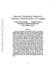
Figure 1. Convolutional networks with adaptive computation graphs (bottom) follow a high level structure similar to Resnets (center). The key difference is that for each layer, a gating function determines in a discrete decision whether to execute or skip the layer. This enables the construction of individual computational graphs based on the input.
featuring a dense connectivity pattern among layers [17] and have performed very large scale experiments to search for optimal architectures using reinforcement learning [44]. While all these models differ in their specific connectivity and architectural details, they have one characteristic in common: a fixed model with an architecture that is agnostic to the input image. A recent study [39] showed that entire layers can be removed from a trained Resnet without harming performance. In fact, almost no individual layer appears critical to the performance. This implies that there is a high degree of redundancy among layers, with many computations potentially rendered unnecessary. This leads us to the following research question. Do we really need a fixed structure for convolutional networks, or could we assemble a network graph on the fly, conditioned on the input? For example, if a network is already confident after a few layers that an image contains a dog, it might jump right to a layer that can distinguish different dog breeds instead of executing all intermediate layers that might be specialized in unrelated aspects.
1. Introduction Deep convolutional networks [25, 26] have enabled a series of major advances for many computer vision problems. Starting with image classification [25, 43], they are now used for many other tasks including object detection [7, 29] and segmentation [12, 30]. In recent years we have seen many improvements upon the original convolutional network architecture. We know that network depth plays a key role for classification performance [34, 37] and that computation can be performed in parallel paths [37]. The seminal work on Resnets [13] showed that adding identity skipconnections bypassing each layer greatly improves gradient propagation, allowing the training of even deeper networks. Most recently, researchers proposed more compact models 1
In this work we present Adanets, convolutional networks with adaptive computation graphs. Figure 1 gives a schematic overview of the proposed approach and highlights the key differences to traditional fixed network architectures. The overall architecture resembles a Resnet in that it contains an information stream from input to output upon which layers compute functions and add the output back to the stream. The main difference is that the set of functions is not fixed. For each residual layer, a gating function determines whether the execution of the layer is required or whether it can be skipped. A key challenge is that the gating functions need to make discrete decisions, which are difficult to integrate into convolutional networks that we would like to train using gradient descent. To incorporate the discrete steps, we build upon recent work [4, 21, 31] that introduces differentiable approximations for discrete stochastic nodes in neural networks. This enables us to model the gating functions as discrete random variables over two states: to execute the next layer or to skip it. To effect the gating based on the input, we model the distribution of the random variables as conditional on the current state of the information stream. This allows the construction of computation graphs adaptively based on the input image and to train both the convolutional weights as well as the discrete gating functions jointly in an end-to-end fashion. In experiments on the CIFAR-10 [24] and ImageNet [5], we demonstrate that Adanets effectively allocate their computational budget among layers. With only 4% additional parameters and 0.04% more computations, Adanets enable adaptive graphs that can skip over 30% of the layers. Further, Adanets learn to generate distinct computational graphs for different high-level categories. On ImageNet some layers exclusively execute for images of animals, whereas other layers focus solely on man-made objects. We further show that Adanets achieve competitive classification performance. On ImageNet, an Adanet based on Resnet 50 achieves a top 5 error of 7.94%, compared to a 7.8% for the full Resnet 50, but at only 67% of the computations. A smaller, but computationally still more expensive Resnet 34 only achieves an error rate of 8.58%. Lastly, we study the effects of adaptive computation on susceptibility to adversarial examples. Adanets exhibit a higher robustness to adversarial attacks than Resnets, complementing other defenses such as JPEG compression.
construct computational graphs based on the input image on the fly, while the convolutional network executes. Our approach can be seen as an example of adaptive computation time for neural networks. Cascaded classifiers [40] have a long tradition for computer vision by quickly rejecting “easy” negatives. Recently, similar approaches have been proposed for neural network based approaches [27, 41]. In an alternative direction, [3, 33] propose to adjust the amount of computation in fully-connected neural networks. To adapt the computation time in convolutional networks, [16, 38] propose network architectures that add classification branches to intermediate layers. This allows one to stop a computation early, once a satisfying level of confidence is reached. Most closely related to our approach is the work on spatially adaptive computation time for residual networks [6]. There, a Resnet adaptively determines after which layer to stop computation. Our work differs from this approach in that we do not perform early stopping and thus do not solely focus on early layers. Instead, in our work for each inference any subset of layers can be selected for execution. This enables the emergence of category-specific computation graphs and also leads to more equal training signals for all layers. Our work is further related to network regularization with stochastic noise. By randomly dropping individual neurons during training, Dropout [35] offers an effective way to prevent neural networks from overfitting. Closely related is the work on stochastic depth [18], where entire layers of a Resnet are randomly removed during each training iteration. Our work resembles this approach in the sense that it also includes stochastic nodes that decide whether to execute or skip layers. In contrast to our work, the layer removal in stochastic depth does not depend on the input image and aims to increase redundancy among layers. In our work, we learn when to skip a layer conditioned on the input image to allow the network to learn layers specialized on subsets of the data. Lastly, our work can also be seen as an example of attention mechanisms in that we select specific layers of importance to assemble the computation graph. This is related to approaches such as highway networks [36] and squeezeand-excitation networks [15], where the output of a residual layer is rescaled according to its importance. This allows these approaches to emphasize some layers and pay less attention to others. In contrast to our work, this still requires the execution of every single layer.
2. Related Work Our study is related to prior work in multiple fields. Several recent works have focused on neural network composition for visual question answering [1, 2, 22] and zeroshot learning [32]. While these approaches include convolutional networks, they focus on constructing a computational graph up front to solve a (mostly visual question answering) task. In contrast, the focus of our work is to
3. Adanets Traditional feed-forward convolutional networks can be considered as a set of N layers, or functions, which are sequentially applied to an input image. Formally, let Fl (·), l ∈ {1, ..., N } denote the function computed by the lth layer. With x0 as input image and xl as output of the lth 2
i.i.d. Gumbel samples
Convolu�onal feature map avg. pool
H×W×C
1×1×C
F(· ,W)
1×1×2
so�max
+
f1
backward
+
go on if argmax is 1
forward
Residual layer with discrete gate
argmax es�ma�ng probabili�es
straight-through Gumbel sampling
Figure 2. Overview of gating unit. The first part estimates the probability for the gate to open. The second part draws a sample form the estimated probability. During the forward pass, we draw a discrete sample using the Gumbel-Max trick. For the backwards pass, we compute the gradient of the softmax-relaxation, allowing us to train the gates and the convolutional layers jointly using gradient descent.
layer, such a network can be recursively defined as xl = Fl (xl−1 )
options: to execute the next layer or to skip it. This allows individual computation graphs per input. This is in contrast to attention mechanisms such as highway networks [36], which share surface resemblance with this formulation. There, the output of a layer is a linear combination of its input and the output computed by the layer’s function: xl = (1 − z(xl−1 )) · xl−1 + z(xl−1 ) · Fl (xl−1 ). The gate acts as a soft attention mechanism that can emphasize certain layers and reduce attention to others. In contrast to our work, this formulation still requires the execution of every single layer.
(1)
Resnets [13] change this definition by introducing identity skip-connections that bypass each layer, i.e., the input to each layer is also added to its output. This has been shown to greatly ease optimization during training. As gradients can propagate directly through the skip-connection, early layers still receive sufficient learning signal even in very deep networks. A Resnet can be defined as xl = xl−1 + Fl (xl−1 )
(2)
3.2. Gating Unit
The introduction of Resnets gave rise to ultra deep networks with over 1000 layers [14, 19]. This drastic increase in network depth motivated a series of experiments [39] investigating the effects of the residual connections and increased network depth. The experiments show that, although all layers are trained jointly, almost any individual layer can be removed from a trained Resnet without harming performance. This surprising phenomenon implies that there is a high degree of independence and redundancy among layers.
Key to the proposed adaptive architecture is the gating function z(xl−1 ). For the gate to be effective, it needs to (1) understand the input features, (2) make a discrete decision, and (3) operate with low computational overhead. We propose a gate that consists of two main components. The first component estimates the probability that the next layer should be executed. The second component takes the estimated probability and draws a discrete sample from it. Figure 2 provides on overview of the proposed gating unit.
3.1. Adaptive Computation Graph
Estimating Probabilities The input to the gate is the convolutional feature map produced by the previous layer xl−1 ∈ RW ×H×C . Operating on the full feature map is computationally expensive and would diminish the benefit of potentially skipping the layer. To build a lightweight gate, we build upon insights by recent studies [15, 20, 28], which show that much of the information in convolutional features is captured by the statistics of the different channels and their interdependencies. To capture as much information from the channel statistics as possible, while remaining computationally efficient, we only consider global channel features. In particular, we perform global average pooling to capture channel-wise means.
Inspired by the observation in [39], we would like to reflect on the way we think about convolutional networks. Do convolutional networks really need a fixed feed-forward structure? Since a fixed structure leads to many redundant computations, could we assemble a network on the fly? An adaptive architecture could have specialized layers and only compute those necessary for the specific input. Consider a network that follows the general principle of a Resnet, but instead of executing all functions, it can determine on an ‘as needed’ basis which layers to execute and which to skip. Such a network can be defined as xl = xl−1 + z(xl−1 ) · Fl (xl−1 )
where z(xl−1 ) ∈ {0, 1}
(3)
where z(xl−1 ) is a gating function that, conditioned on the input to the layer, makes a decision between two discrete
zc =
3
H X W X 1 xi,j,c H × W i=1 j=1
(4)
This compresses the input features into a 1×1×C channel descriptor. We follow the pooling step with a second operation to capture the dependencies between the channels. The output of that operation is a two-dimensional vector β containing the log-probabilities for computing and skipping the following layer, respectively. We opt for a simple nonlinear function that consists of two fully-connected layers connected with a ReLU [8] activation function.
ˆ k = softmax ((log αk + Gk ) /τ ) X
ˆ k is the k th element in X ˆ and τ is the temperawhere X ture of the softmax operation. With τ → 0, the softmax function approaches the argmax function and Equation 7 becomes equivalent to the discrete sampler. For τ → ∞ it becomes a uniform distribution. Since the softmax function is differentiable and Gk is an independent noise term, we can easily propagate gradients to the probabilities αk . This enables the gating function to receive learning signals for when to open and when to close. To generate samples, we set the log probabilities to be the output of the gate’s first component so that log α = β. One option to employ the Gumbel-softmax estimator is to use the continuous version from Equation 7 during training and obtain discrete samples with Equation 6 during testing. This would allow us to train the network end-to-end using gradient descent and have sparse inference at test time. An alternative is the straight-through version [21] of the Gumbel-softmax estimator. There, during training, for the forward pass we get discrete samples from Equation 6, but during the backwards pass we compute the gradient of the softmax relaxation in Equation 7. Note that the estimator is biased due to the mismatch between forward and backward pass. However, we observe that empirically the greedy straight-through estimator performs better and further leads to computational graph structures that are more categoryspecific. We illustrate the two different paths during the forward and backward pass in Figure 2.
(5)
β = W2 σ(W1 z) C d
and W2 ∈ where σ refers to the ReLU, W1 ∈ R C R2× d . To further limit computation, we reduce the dimensionality after the first layer by a factor d. The lightweight design of the gating function leads to minimal computational overhead. For an Adanet based on Resnet 110 for CIFAR-10, gating accounts for only 0.01% additional computations. For an Adanet based on Resnet 50 for ImageNet, the gating function accounts for only 0.04%, but allows us to skip 33% of layers on average. ×C
Greedy Gumbel Sampling After estimating the logprobabilities β, a key challenge for the proposed architecture is that the gating function z(xl−1 ) needs to make a discrete decision. However, discrete decisions are nondifferentiable and as such cannot be simply incorporated in a convolutional architecture that we would like to train using gradient descent. To bridge the discrete step, we build upon recent works that propose approaches for propagating gradients trough stochastic neurons [4, 23]. In this work, we utilize the Gumbel-Max trick [10] and in particular its recent continuous relaxation [21, 31]. A random variable G is defined to follow a Gumbel distribution if G = − log(− log(U )), with U being a sample from the uniform distribution U ∼ Unif[0, 1]. For our work it is key that we can parameterize discrete distributions in terms of Gumbel random variables. In particular, let X be a discrete random variable with probabilities P (X = k) ∝ αk and let {Gk }k∈{1,...,K} be a sequence of i.i.d. Gumbel random variables. Then, we can sample from the discrete variable with X = arg max (log αk + Gk )
(7)
3.3. Training Adanets The adaptive gating functions require a few considerations that are absent in plain Resnets: • Without proper training incentives, Adanets might not learn effective computational graphs and default to trivial solutions, e.g., always using all layers. • If gates turn off too frequently, the network could face the dead layer problem [6], i.e., some layers would not receive enough training signal and atrophy.
(6)
• Since each image is processed by a different set of layers, the effective batchsize for each layer is reduced [33], which could disrupt learning.
k∈{1,...,K}
The drawback of this approach is that the argmax operation that maps the Gumbel samples to the realizations of the discrete distribution is not continuous. To address this, a continuous relaxation of the Gumbel Sampling Trick has been proposed [21, 31], replacing the argmax operation with a softmax. Note that a discrete random variable can be expressed as a one-hot vector, where the realization of the variable is the index of the non-zero entry of the vector. With this notation, a sample from the Gumbel softmax ˆ as follows: relaxation can be expressed by the vector X
Since the key goal is to classify images correctly, the main training loss is a basic multi-class logistic loss that we denote as LM C . Further, we would like the network to learn how to allocate computation among layers effectively. One option would be a penalty on the total computation. We observe this does not lead to effective computation graphs. The network quickly defaults to shutting off some layers, reducing itself to a plain Resnet with fewer layers. 4
0.9
8
classes
Table 1. Test error on CIFAR 10 in % for Resnets, wide Resnets and their adaptive Adanet counterparts. Adanet 110 clearly outperforms Resnet 110 while only using a subset of the layers.
execution rates
downsampling
Adanet 110:
Model
6 0.8
4 2 0
0.7 0
20
residual layers
Wide Adanet 89:
40
downsampling 0.9
classes
8 6
0.65
4
0.4
0
10
residual layers
20
l=1
(z l − t)
Resnet 110 [13] Pre-Resnet [14] Stochastic Depth [19] Adanet 110 Adanet 110*
6.61 6.37 5.25 5.76 5.14
1.7M 1.7M 1.7M 1.78M 1.78M
0.5 0.5 0.5 0.41 0.5
Wide Resnet (4x width) [42] Wide Resnet (10x width) [42] Wide Adanet 89 Wide Adanet 89*
4.53 4.0 4.46 3.88
8.7M 36.5M 36.1M 36.1M
2.6 10.49 1.6 2.13
We perform a series experiments to evaluate the performance of Adanets and how effectively they assign computational budget among layers. Further, we investigate whether they learn specialized layers and category-specific computational graphs. Lastly, we look beyond performance and study the robustness of Adanets by analyzing their effect on the susceptibility towards adversarial attacks.
We propose an alternative loss function, where, instead of penalizing every computation, we encourage each layer to be executed at a certain target rate t. In particular, we approximate the execution rate for each layer over a minibatch and penalize deviations from the target rate. Let z l denote the fraction of times layer l is executed within a minibatch. Then, the target rate loss is defined as N X
GFLOPs
4. Experiments
Figure 3. Execution rates per layer and class on CIFAR-10. We observe that downsampling layers are of key importance and have the highest execution rates. Further, the wide Adanet exhibits substantially more variation between the classes and later layers perform more class specific operations compared to earlier layers.
Ltarget =
#Params
time to model the data, before the gates need to become discriminative. Over the course of training, the learning rates of the convolutional layers and the gates align.
2 0
Error
2
4.1. Results on CIFAR We first perform a set of experiments on CIFAR-10 [24] to validate the gating mechanism and how effectively Adanets distribute computation among layers. Model configurations First, we construct a basic Adanet 110 from the standard Resnet 110 [13]. The reduction rate is set to d = 2, resulting in a computational overhead of only 0.01% and 4.8% more parameters. Further, we use a wide Adanet with substantially more parameters with 3, 4, 20 and 2 bottleneck blocks at four scales with 64, 128, 256 and 512 channels per block respectively. For the wide Adanet we use a reduction rate of d = 16, leading to a gating overhead of 0.14%. We compare standard Adanets, i.e., only execute layers with open gates, to a second variant indicated by “ ∗ ”, where analogous to Dropout [35] and stochastic depth [19] all layers are executed and their output is scaled by the expected execution rate.
(8)
The target rate provides an easy instrument to adjust the desired computation time. We use a target rate of t = 0.6, but we generally observe good performance when t ≥ 0.5. When t is far below 0.5, the effective batchsize per layer gets too small and disrupts training. With the target rate loss and multi-class loss, the overall training loss for Adanets is LAdanet = LM C + λLtarget
(9)
where λ trades-off between the different loss terms. In our experiments, we choose λ = 2. To prevent layers from reaching extreme states in early training, such as never being executed, we propose two design choices. First, we initialize the gates to be biased towards opening. This ensures that all layers receive sufficient learning signal in early training. Second, we reduce the learning rate of the gates. This gives the layers more
Training details We follow a similar training scheme as [13] and train all models using stochastic gradient descent. We use momentum with weight of 0.9 and adopt a weight decay of 5 × 10⁻⁴ . All models are trained for 350 epochs with a mini-batch size of 256. We use a step-wise learning rate starting at 0.1 and decaying by 10−1 after 150 5
Table 2. Test error on ImageNet in % for Adanet 50 and several Resnets of varying depths. Adanet 50 clearly outperforms the computationally more expensive ResNet 34. Top 1
Top 5
#Params
GFLOPs
Resnet 18 [13] Resnet 34 [13] Resnet 50 [13] Adanet 50
30.24 26.69 24.7 25.38
10.92 8.58 7.8 7.94
11.69 21.8 25.56 26.56
1.8 3.6 3.8 2.57
Frequency
Model
birds consumer goods all classes
0.4 0.35 0.3 0.25 0.2 0.15 0.1 0.05 0
and 250 epochs. For the gates, the learning rate starts from 2 × 10⁻⁴ and decays by 4 × 10⁻¹ . Gates are initialized to open at a rate of 85% at the beginning of training. We adopt a standard data-augmentation scheme, where images are padded with 4 pixels on each side, randomly cropped to 32 × 32 and with probability 0.5 horizontally flipped.
6
8
10
12
14
16
Number of layers
Figure 4. Distribution of number of executed layers. On ImageNet, 10.8 layers are executed in average. Generally, images of animals use fewer layers compared to man-made objects.
4.2. Results on ImageNet In a second set of experiments, we study the differences between the computational graphs of different categories. Since CIFAR-10 has a limited variety of object categories, we evaluate Adanets on the ImageNet [5] dataset.
Quantitative comparison Table 1 shows the classification results on CIFAR 10 for standard Resnets [13], wide Resnets [42] and their adaptive Adanet counterparts. From the results, we observe that Adanets clearly outperform their Resnet counterparts. Even the Adanet 110 that only uses a subset of the layers achieves a better performance than Resnet 110. The competitive performance indicates that it is indeed possible to train a convolutional network with adaptive computation graph end-to-end using gradient descent. Further, the proposed adaptive gating architecture appears to be an effective means to reduce computation.
Model and training details We construct an Adanet 50 based on Resnet 50 [13]. We choose a reduction rate of d = 16, adding only 3.9% more parameters and a computational overhead of 0.04%. As before, we train the model using stochastic gradient descent with a mini-batch size of 256. Further, we use momentum with a weight of 0.9 and adopt a weight decay of 10−4 . Due to the reduced effective batch-size, we increase the number of epochs from the standard Resnet training schedule. The model is trained for 130 epochs, with a step-wise learning rate which starts at 0.1 and decays be 10−1 every 40 epochs. As for CIFAR-10, the learning rates of the gates starts from 2 × 10⁻⁴ and decays by steps of 4 × 10⁻¹ . The gates are initialized to open at a rate of 85% in the beginning of training. During training, we use the data-augmentation procedure as in [13], at test time, we first rescale images to 256 × 256 followed by a 224 × 224 center crop.
Analysis of learned computational graphs To investigate how the network allocates computation, we look at the rate at which different layers are executed for images of different categories. Figure 3 shows a histogram of the execution rates for Adanet 110 on top and for Wide Adanet 89 on the bottom. The x-axis shows the residual layers and the yaxis shows the 10 classes in CIFAR-10. From the figure we make three main observations. First, downsampling layers deviate significantly from the target execution rate. Specifically, they are executed substantially more often than other layers, indicating their key role in the network [39]. Second, the wide Adanet 101 shows substantially more variation between classes, indicating that more capacity might help individual layers specialize on certain subsets of the data. Third, most inter-class variation comes from later layers of the network. This behavior could arise due to multiple reasons. On one hand, early layers might comprise generic functions useful to all categories. On the other hand, they might not yet capture sufficient semantic information to discriminate between categories. Further, due to their larger spatial resolution, less information might be captured in the global channel statistics used by the gating function.
Quantitative comparison Table 2 shows the classification results on ImageNet for Adanet 50 and several Resnets of varying depth. Adanet 50 substantially reduces the computational cost by 33% compared to Resnet 50 with only minimal reduction in performance. Moreover, Adanet 50 significantly outperforms the smaller, but computationally more expensive, Resnet 34. This demonstrates the effectiveness of Adanets in reducing computation without sacrificing much performance. Further, we again perform an evaluation, in which we execute all layers and scale their output by the expected execution rate. Interestingly, we do not observe changes in performance. This indicates Adanets successfully learn specialized layers on ImageNet instead of replicas of similar functions. 6
Adanet 50:
1
downsampling
Frequency of execution
food plants consumer goods
container
equipment structure
man-made objects
furnishing
ImageNet classes
dogs
animals
birds insects reptiles fish other animals others 15
execution rates
0
0.25
0.5
0.75
other layers 0.8 0.7 0.6
10
epochs
20
30
serve downsampling layers are again of key importance, and further the last layer also takes a key role. Third, we see a clear distinction between man-made objects and animals. Specifically, layers 9, 10 and 14 seem to specialize in man-made objects, whereas layers 8, 11 and 12 focus on animals. Moreover, we even observe distinct differences between mid-level categories such as mammals, birds and insects. It is worthy of note that the training objective does not include an incentive to learn category specific layers. The specialization appears to emerge naturally when the computational budget gets constrained. Fourth, the classspecificity is again higher for layers positioned later in the network. Further, although layers 8 to 12 exhibit a much larger variance in execution rates, their average rate is similar to early layers and close to the target rate of 0.6. The layers are initialized to execute a rate of 85% at the start of training. Figure 6 shows a typical trajectory of the execution rates over the first 30 training epochs, after which, the rates stay roughly the same. The figure shows that the layers are quickly separated into key layers and less critical layers, although the gates are updated with a much lower learning rate. Important layers such as downsampling and the last layers increase their execution rate, while the remaining layers slowly approach the target rate.
cats
5 10 residual layers
downsampling layers
Figure 6. Execution rates per layer over the first 30 epochs on ImageNet. Layers are quickly separated. Downsampling layers and the last layer increase their execution rate, while the remaining layers slowly approach the target rate.
other objects
0
0.9
0.5 0
transport
other mammals
last layer second last layer
1
Figure 5. Execution rates per layer and class on ImageNet. We observe that some downsampling layers and the last layer are executed for all images. Further, we see clear differences between the execution rates for images of animals and man-made objects. Even some mid-level categories such as mammals, birds and insects show distinct patterns.
Variable inference time Due to the adaptive computation graphs each inference path might be different. As a consequence computation time varies across different images. Figure 4 shows the distribution of how many layers are executed over all ImageNet validation images. On average 10.81 layers are executed with a standard deviation of 1.11. The figure also shows the distributions for the mid-level categories of birds and consumer goods. In expectation, images of birds use one layer less than images of consumer goods. Further, from Figure 5 we also know that the two groups not only use different numbers of layers, but also different sets of layers.
Analysis of learned computational graphs Similar to above, Figure 5 shows the execution rates for the layers in Adanet 50 broken down by the 1000 classes in ImageNet. On the right, the figure shows high-level and mid-level categories that contain large numbers of classes. From the figure we make four main observations. First, we observe a much wider range of execution rates ranging from 0 to 1. Three layers are always used and layers 9 and 10 are only rarely used for a large subsets of classes. Second, we ob7
Fast Gradient Sign Method Adanet 50 Adanet 50 + JPEG compression Resnet 50 Resnet 50 + JPEG compression
0.7 0.6
Top 1 accuracy
1
Frequency of execution
0.8
0.5 0.4 0.3
birds birds FGSM (epsilon 0.047)
0.8
target rate
0.6 0.4 0.2 0
0
0.2
10
15
Residual layers
0.1 0 0
5
0.01
0.02
0.03
0.04
0.05
Figure 8. Effect of adversarial attack on execution rates of layers over all classes of birds. The execution rates remain mostly unaffected by the attack.
0.06
Adversary strength (epsilon)
ter performing an FGSM attack with epsilon 0.047. We choose birds because they account for a substantial amount of classes and because they show a distinct gating pattern. The results show that, although the accuracy of the network drops from 74.62% to just over 11%, the execution rates remain similar. The resilience of the gating towards the attack might arise from multiple reasons. First, the gating for layers that are always used might rely mostly on the gates’ bias that is independent on the input. Second, the global average pooling might balance out some of the adversarial perturbations. Lastly, the stochasticity induced by the Gumbel noise might outweigh the changes from the attack.
Figure 7. Adversarial attack using Fast Gradient Sign Method on plain Resnets and Adanets. We observe that Adanets are consistently more robust. Further, the additional robustness persists even when additional defense mechanisms are applied.
4.3. Robustness to adversarial attacks In a third set of experiments we aim to understand the effect of adaptive computation graphs on the susceptibility towards adversarial attacks. We have seen that Adanets learn specialized layers and category-specific computational graphs. In the scenario of an adversarial attack, it becomes unclear, whether the adaptive gating helps or harms the robustness. On the one hand, if adversarial perturbations lead to key layers of the network to be skipped, performance might degrade. On the other hand, the stochasticity of the graph might improve robustness. To shed light on this question, we perform a Fast Gradient Sign Attack [9] on Resnet 50 and Adanet 50, both trained on ImageNet. The results are shown in Figure 7. On the x-axis we show the strength of the adversary as measured in epsilon, i.e., the amount each pixel is allowed to be changed. On the y-axis we report the top-1 classification accuracy on ImageNet. We observe the Adanet is consistently more robust, independent of adversary strength. To investigate whether this additional robustness complements other known defenses [11], we perform a follow-up experiment in which we perform JPEG compression on the adversarial examples. We follow [11] and use a JPEG quality setting of 75%. The figure shows that both networks greatly benefit from the JPEG compression defense. Further, Adanet 50 remains more robust than Resnet 50 indicating the additional robustness can complement other defenses. To further the understanding of the effect of the adversarial attack on the proposed gating mechanism, we look at the execution rates of the layers before and after the attack. Specifically, Figure 8 shows the average execution rates over all bird categories for Adanet 50 before and af-
5. Conclusion In this work, we introduced Adanets: convolutional networks with adaptive computation graphs. Adanets can determine for each input adaptively which layers of the network to execute. In a range of experiments on CIFAR-10 and ImageNet, we demonstrated that Adanets are an effective means to reduce computation time without compromising much on performance. Further, Adanets learn to specialize layers on distinct subsets of the data and to generate distinct category-sepecific computational graphs. Lastly, we showed that Adanets exhibit a larger robustness towards adversarial examples compared to their plain Resnet counterparts. This robustness advantage appears to remain, even after applying additional defense mechanisms. This work opens up numerous paths for future work. For example, with respect to network architecture, it would be intriguing to extend this work beyond Resnets to other high-level architectures such as densely-connected [17] or inception-based [37] networks. Further, it would be interesting to investigate Adanets for other tasks such as image segmentation or object detection. Along those lines, the gates in Adanets perform global average pooling to aggregate input features. This step might limit the effectiveness when dealing with large spatial resolutions, which are common for image segmentation. It would be interesting 8
to study the effect of different aggregation methods on the different layers in the network. From an optimization perspective, we have seen that layers take on different roles in Adanets. Future work could study whether one should treat the layers differently during training to further improve their effectiveness. From a practitioner’s point of view, it might be dissatisfying that Adanets have varying inference times. It would be exciting to extend this work into a framework where the set of executed layers is adaptive, but their number is fixed. Lastly, we have seen that the gating functions are largely unaffected by basic adversarial attacks. For an adversary, it could be interesting to investigate attacks that specifically target the gating functions.
[9] I. J. Goodfellow, J. Shlens, and C. Szegedy. Explaining and harnessing adversarial examples. arXiv preprint arXiv:1412.6572, 2014. [10] E. J. Gumbel. Statistical theory of extreme values and some practical applications: a series of lectures. Number 33. US Govt. Print. Office, 1954. [11] C. Guo, M. Rana, M. Cisse, and L. van der Maaten. Countering adversarial images using input transformations. arXiv preprint arXiv:1711.00117, 2017. [12] K. He, G. Gkioxari, P. Doll´ar, and R. Girshick. Mask r-cnn. ICCV, 2017. [13] K. He, X. Zhang, S. Ren, and J. Sun. Deep residual learning for image recognition. In Proceedings of the IEEE conference on computer vision and pattern recognition, pages 770–778, 2016. [14] K. He, X. Zhang, S. Ren, and J. Sun. Identity mappings in deep residual networks. In European Conference on Computer Vision, pages 630–645. Springer, 2016. [15] J. Hu, L. Shen, and G. Sun. Squeeze-and-excitation networks. arXiv preprint arXiv:1709.01507, 2017. [16] G. Huang, D. Chen, T. Li, F. Wu, L. van der Maaten, and K. Q. Weinberger. Multi-scale dense convolutional networks for efficient prediction. arXiv preprint arXiv:1703.09844, 2017. [17] G. Huang, Z. Liu, K. Q. Weinberger, and L. van der Maaten. Densely connected convolutional networks. CVPR, 2017. [18] G. Huang, Y. Sun, Z. Liu, D. Sedra, and K. Q. Weinberger. Deep networks with stochastic depth. In European Conference on Computer Vision, pages 646–661. Springer, 2016. [19] G. Huang, Y. Sun, Z. Liu, D. Sedra, and K. Q. Weinberger. Deep networks with stochastic depth. In European Conference on Computer Vision, pages 646–661. Springer, 2016. [20] X. Huang and S. Belongie. Arbitrary style transfer in realtime with adaptive instance normalization. arXiv preprint arXiv:1703.06868, 2017. [21] E. Jang, S. Gu, and B. Poole. Categorical reparameterization with gumbel-softmax. arXiv preprint arXiv:1611.01144, 2016. [22] J. Johnson, B. Hariharan, L. van der Maaten, J. Hoffman, L. Fei-Fei, C. L. Zitnick, and R. Girshick. Inferring and executing programs for visual reasoning. arXiv preprint arXiv:1705.03633, 2017. [23] D. P. Kingma and M. Welling. Auto-encoding variational bayes. arXiv preprint arXiv:1312.6114, 2013. [24] A. Krizhevsky and G. Hinton. Learning multiple layers of features from tiny images. 2009. [25] A. Krizhevsky, I. Sutskever, and G. E. Hinton. Imagenet classification with deep convolutional neural networks. In Advances in neural information processing systems, pages 1097–1105, 2012. [26] Y. LeCun, L. Bottou, Y. Bengio, and P. Haffner. Gradientbased learning applied to document recognition. Proceedings of the IEEE, 86(11):2278–2324, 1998. [27] H. Li, Z. Lin, X. Shen, J. Brandt, and G. Hua. A convolutional neural network cascade for face detection. In Proceedings of the IEEE Conference on Computer Vision and Pattern Recognition, pages 5325–5334, 2015.
Acknowledgements We would like to thank Daniel D. Lee, Ilya Kostrikov and Antonio Marcedone for insightful discussions and feedback. This work was supported in part by the AOL Connected Experiences Laboratory, a Google Focused Research Award, AWS Cloud Credits for Research and a Facebook equipment donation.
References [1] J. Andreas, M. Rohrbach, T. Darrell, and D. Klein. Learning to compose neural networks for question answering. arXiv preprint arXiv:1601.01705, 2016. [2] J. Andreas, M. Rohrbach, T. Darrell, and D. Klein. Neural module networks. In Proceedings of the IEEE Conference on Computer Vision and Pattern Recognition, pages 39–48, 2016. [3] E. Bengio, P.-L. Bacon, J. Pineau, and D. Precup. Conditional computation in neural networks for faster models. arXiv preprint arXiv:1511.06297, 2015. [4] Y. Bengio, N. L´eonard, and A. Courville. Estimating or propagating gradients through stochastic neurons for conditional computation. arXiv preprint arXiv:1308.3432, 2013. [5] J. Deng, W. Dong, R. Socher, L.-J. Li, K. Li, and L. FeiFei. Imagenet: A large-scale hierarchical image database. In Computer Vision and Pattern Recognition, 2009. CVPR 2009. IEEE Conference on, pages 248–255. IEEE, 2009. [6] M. Figurnov, M. D. Collins, Y. Zhu, L. Zhang, J. Huang, D. Vetrov, and R. Salakhutdinov. Spatially adaptive computation time for residual networks. arXiv preprint arXiv:1612.02297, 2016. [7] R. Girshick, J. Donahue, T. Darrell, and J. Malik. Rich feature hierarchies for accurate object detection and semantic segmentation. In Proceedings of the IEEE conference on computer vision and pattern recognition, pages 580–587, 2014. [8] X. Glorot, A. Bordes, and Y. Bengio. Deep sparse rectifier neural networks. In Proceedings of the Fourteenth International Conference on Artificial Intelligence and Statistics, pages 315–323, 2011.
9
[28] Y. Li, N. Wang, J. Liu, and X. Hou. Demystifying neural style transfer. arXiv preprint arXiv:1701.01036, 2017. [29] T.-Y. Lin, P. Doll´ar, R. Girshick, K. He, B. Hariharan, and S. Belongie. Feature pyramid networks for object detection. In Computer Vision and Pattern Recognition (CVPR), Honolulu, HI, 2017. [30] J. Long, E. Shelhamer, and T. Darrell. Fully convolutional networks for semantic segmentation. In Proceedings of the IEEE Conference on Computer Vision and Pattern Recognition, pages 3431–3440, 2015. [31] C. J. Maddison, A. Mnih, and Y. W. Teh. The concrete distribution: A continuous relaxation of discrete random variables. arXiv preprint arXiv:1611.00712, 2016. [32] I. Misra, A. Gupta, and M. Hebert. From red wine to red tomato: Composition with context. CVPR, 2017. [33] N. Shazeer, A. Mirhoseini, K. Maziarz, A. Davis, Q. Le, G. Hinton, and J. Dean. Outrageously large neural networks: The sparsely-gated mixture-of-experts layer. arXiv preprint arXiv:1701.06538, 2017. [34] K. Simonyan and A. Zisserman. Very deep convolutional networks for large-scale image recognition. arXiv preprint arXiv:1409.1556, 2014. [35] N. Srivastava, G. E. Hinton, A. Krizhevsky, I. Sutskever, and R. Salakhutdinov. Dropout: a simple way to prevent neural networks from overfitting. Journal of machine learning research, 15(1):1929–1958, 2014. [36] R. K. Srivastava, K. Greff, and J. Schmidhuber. Highway networks. arXiv preprint arXiv:1505.00387, 2015. [37] C. Szegedy, W. Liu, Y. Jia, P. Sermanet, S. Reed, D. Anguelov, D. Erhan, V. Vanhoucke, and A. Rabinovich. Going deeper with convolutions. In Proceedings of the IEEE conference on computer vision and pattern recognition, pages 1–9, 2015. [38] S. Teerapittayanon, B. McDanel, and H. Kung. Branchynet: Fast inference via early exiting from deep neural networks. In Pattern Recognition (ICPR), 2016 23rd International Conference on, pages 2464–2469. IEEE, 2016. [39] A. Veit, M. J. Wilber, and S. Belongie. Residual networks behave like ensembles of relatively shallow networks. In Advances in Neural Information Processing Systems, pages 550–558, 2016. [40] P. Viola and M. J. Jones. Robust real-time face detection. International journal of computer vision, 57(2):137–154, 2004. [41] F. Yang, W. Choi, and Y. Lin. Exploit all the layers: Fast and accurate cnn object detector with scale dependent pooling and cascaded rejection classifiers. In Proceedings of the IEEE Conference on Computer Vision and Pattern Recognition, pages 2129–2137, 2016. [42] S. Zagoruyko and N. Komodakis. Wide residual networks. arXiv preprint arXiv:1605.07146, 2016. [43] M. D. Zeiler and R. Fergus. Visualizing and understanding convolutional networks. In European conference on computer vision, pages 818–833. Springer, 2014. [44] B. Zoph, V. Vasudevan, J. Shlens, and Q. V. Le. Learning transferable architectures for scalable image recognition. arXiv preprint arXiv:1707.07012, 2017.
10