Inside the. PostgreSQL Query Optimizer. Neil Conway
.
Fujitsu Australia Software Technology. PostgreSQL Query Optimizer Internals – p
. 1 ...
Inside the PostgreSQL Query Optimizer Neil Conway
[email protected]
Fujitsu Australia Software Technology
PostgreSQL Query Optimizer Internals – p. 1
Outline Introduction to query optimization Outline of query processing Basic planner algorithm Planning specific SQL constructs Questions welcome throughout
PostgreSQL Query Optimizer Internals – p. 2
What is query optimization? SQL is declarative; the user specifies what the query returns, not how it should be executed There are many equivalences in SQL: Joins can be applied in any order Predicates can be evaluated in any order Subselects can be transformed into joins Several different methods of doing the same operation: Three core join algorithms (nested loops, hash join, merge join) Two aggregation algorithms (hashing, sorting) Two scan algorithms (index scan, sequential scan) For a non-trivial query there are many alternative plans PostgreSQL Query Optimizer Internals – p. 3
Outline of query processing Client connects to postmaster via TCP or unix domain socket, communicates via frontend-backend protocol fork new backend to handle connection
Authentication in new backend Enter simple query loop Client submits query Backend executes query, returns result set
PostgreSQL Query Optimizer Internals – p. 4
Query loop 1. Lex and parse — flex, bison Input: query string Output: “raw parsetree” No database access or semantic analysis 2. Analysis Input: raw parsetree Output: Query Essentially, annotated parsetree — do database lookups for metadata 3. Rewriter Input: Query Output: One or more Query Apply rewrite rules: CREATE RULE, CREATE VIEW PostgreSQL Query Optimizer Internals – p. 5
Query loop, cont. Already done: we understand the syntax of the query and have looked up associated metadata and applied some basic semantic checks If this is a “utility command” (CREATE, ALTER, DROP, etc.), hand off to the implementation of the command Otherwise, remaining work: Decide how to evaluate the query, produce a Plan Evaluate the Plan and return result set to client The query planner is what determines the best way to evaluate a query; also known as the “query optimizer”. This requires: 1. Determining the set of possible plans 2. Choosing the “best” plan from this set PostgreSQL Query Optimizer Internals – p. 6
Representation of query plans We represent “how” to execute a query as a tree of plan nodes; each node is a single operation (join, disk scan, sort, etc.) Tuples flow from the leaves of the tree (disk scans) up to the root Results delivered to parent node “on demand” To get a row, a node “pulls” on its child node, which in turns pulls on its child nodes as needed To produce result set, executor just pulls on root node Guts of query execution is in the implementation of plan nodes In general, plan nodes are asymmetric: left and right inputs treated differently PostgreSQL Query Optimizer Internals – p. 7
Example query Database stores CVS commit history A commit modifies n files; each such modification is an “action” Query: find the timestamp of the latest commit to modify given a file f SELECT c.tstamp FROM commits c, actions a WHERE a.file IN (SELECT id FROM files WHERE path = ’...’) AND a.commit_id = c.id ORDER BY c.tstamp DESC LIMIT 1;
target list range table qualifier IN-clause subquery join predicate sort order limit expression PostgreSQL Query Optimizer Internals – p. 8
Example query plan LIMIT
SORT key: commits.tstamp
JOIN method: nested loops key: action.commit_id = commit.id
JOIN method: nested loops key: file.id = action.file
AGGREGATE method: hashing key: files.id
SCAN commits method: index scan key: id = LEFT.commit_id
SCAN actions method: index scan key: file = LEFT.id
SCAN files method: index scan key: path = ‘...’
PostgreSQL Query Optimizer Internals – p. 9
What makes a good plan? The planner chooses between plans based on their estimated cost Assumption: disk IO dominates the cost of query processing. Therefore, pick the plan that requires least disk IO Random IO is (much) more expensive than sequential IO on modern hardware Estimate I/O required by trying to predict the size of intermediate result sets, using database statistics gathered by ANALYZE This is an imperfect science, at best Distinguish between “startup cost” (IOs required for first tuple) and “total cost” PostgreSQL Query Optimizer Internals – p. 10
General optimization principles The cost of a node is a function of its input: the number of rows produced by child nodes and the distribution of their values. Therefore: 1. Reordering plan nodes changes everything 2. A poor choice near the leaves of the plan tree could spell disaster Keep this in mind when debugging poorly performing plans 3. Apply predicates early, so as to reduce the size of intermediate result sets Worth keeping track of sort order — given sorted input, certain plan nodes are cheaper to execute Planning joins effectively is essential PostgreSQL Query Optimizer Internals – p. 11
Planner algorithm Conceptually, three phases: 1. Enumerate all the available plans 2. Assess the cost of each plan 3. Choose the cheapest plan Naturally this would not be very efficient “System R algorithm” is commonly used — a dynamic programming algorithm invented by IBM in the 1970s Basic idea: find “good” plans for a simplified query with n joins. To find good plans for n + 1 joins, join each plan with an additional relation. Repeat
PostgreSQL Query Optimizer Internals – p. 12
System R algorithm 1. Consider each base relation. Consider sequential scan and available index scans, applying predicates that involve this base relation. Remember: Cheapest unordered plan Cheapest plan for each sort order 2. While candidate plans have fewer joins than required, join each candidate plan with a relation not yet in that plan. Retain: Cheapest unordered plan for each distinct set of relations Cheapest plan with a given sort order for each distinct set of relations
PostgreSQL Query Optimizer Internals – p. 13
System R algorithm, cont. Grouping (aggregation) and sorting is done at the end Consider “left-deep”, “bushy”, and “right-deep” plans (some planners only consider left-deep plans) JOIN
JOIN JOIN
JOIN
A
A JOIN
JOIN
JOIN
B
B A
C
D
JOIN
B
C
JOIN
D
C
D
The number of plans considered explodes as the number of joins increases; for queries with many joins (≥ 12 by default), a genetic algorithm is used (“GEQO”) Non-exhaustive, non-deterministic search of possible left-deep join orders PostgreSQL Query Optimizer Internals – p. 14
Planning outer joins Outer join: like an inner join, except include unmatched join tuples in the result set Inner join operator is both commutative and associative: A 1 B ≡ B 1 A, A 1 (B 1 C) ≡ (A 1 B) 1 C In general, outer joins are neither associative nor commutative, so we can’t reorder them Main difference is fewer options for join order; a pair of relations specified by OUTER JOIN is effectively a single base relation in the planner algorithm Sometimes outer joins can be converted to inner joins: SELECT * FROM a LEFT JOIN b WHERE b.x = k Tip: you can force join order for inner joins by using JOIN syntax with join_collapse_limit set to 1 PostgreSQL Query Optimizer Internals – p. 15
Planning subqueries Three types of subqueries: IN-clause, FROM-list, and expression We always “pull up” IN-clause subqueries to become a special kind of join in the parent query We try to pull up FROM-list subqueries to become joins in the parent query This can be done if the subquery is simple: no GROUP BY, aggregates, HAVING, ORDER BY Otherwise, evaluate subquery via separate plan node (SubqueryScan) — akin to a sequential scan
PostgreSQL Query Optimizer Internals – p. 16
FROM-list subquery example SELECT * FROM t1, (SELECT * FROM t2 WHERE t2.x = 10) t2 WHERE t1.id = t2.id; -- converted by the optimizer into SELECT * FROM t1, t2 WHERE t1.id = t2.id and t2.x = 10;
Subquery pullup allows the planner to reuse all the machinery for optimizing joins Integrating subquery qualifiers into the parent query can mean we can optimize the parent query better
PostgreSQL Query Optimizer Internals – p. 17
Planning expression subqueries Produce nested Plan by recursive invocation of planner An “uncorrelated” subquery does not reference any variables from its parent query; it will therefore remain constant for a given database snapshot. SELECT foo FROM bar WHERE bar.id = (SELECT baz.id FROM baz WHERE baz.quux = 100);
If uncorrelated, only need to evaluate the subquery once per parent query $var = SELECT id FROM baz WHERE quux = 100; SELECT foo FROM bar WHERE id = $var;
If correlated, we need to repeatedly evaluate the subquery during the execution of the parent query PostgreSQL Query Optimizer Internals – p. 18
Planning functions Planner mostly treats functions as “black boxes” For example, set-returning functions in the FROM list are represented as a separate plan node (FunctionScan) Can’t effectively predict the cost of function evaluation or result size of a set-returning function We can inline a function call if: Defined in SQL Used in an expression context (not FROM list — room for improvement) Sufficiently simple: “SELECT ...” If invoked with all-constant parameters and not marked “volatile”, we can preevaluate a function call PostgreSQL Query Optimizer Internals – p. 19
Function inlining example CREATE FUNCTION mul(int, int) RETURNS int AS ‘SELECT $1 * $2’ LANGUAGE sql; SELECT * FROM emp WHERE mul(salary, age) > 1000000; -- after function inlining, essentially SELECT * FROM emp WHERE (salary * age) > 1000000;
The inlined form of the query allows the optimizer to look inside the function definition to predict the number of rows satisfied by the predicate Also avoids function call overhead, although this is small anyway PostgreSQL Query Optimizer Internals – p. 20
Planning set operations Planning for set operations is somewhat primitive Generate plans for child queries, then add a node to concatenate the result sets together Some set operations require more work: UNION: sort and remove duplicates EXCEPT [ ALL ], INTERSECT [ ALL ]: sort and remove duplicates, then produce result set via a linear scan Note that we never consider any alternatives, so planning is pretty simple (patches welcome)
PostgreSQL Query Optimizer Internals – p. 21
Potential improvements Hard: Database statistics for correlation between columns Function optimization Rewrite GEQO Crazy: Online statistics gathering Executor → optimizer online feedback Parallel query processing on a single machine (one query on multiple CPUs concurrently) Distributed query processing (over the network)
PostgreSQL Query Optimizer Internals – p. 22
Questions? Thank you.
PostgreSQL Query Optimizer Internals – p. 23
Using EXPLAIN EXPLAIN prints the plan chosen for a given query, plus the estimated cost and result set size of each plan node
Primary planner debugging tool; EXPLAIN ANALYZE compares planner’s guesses to reality Executes the query with per-plan-node instrumentation
PostgreSQL Query Optimizer Internals – p. 24
EXPLAIN output EXPLAIN ANALYZE SELECT c.tstamp FROM commits c, actions a WHERE a.file IN (SELECT id FROM files WHERE path = ‘...’) AND a.commit_id = c.id ORDER BY c.tstamp DESC LIMIT 1; Limit (cost=135.79..135.80 rows=1 width=8) (actual time=4.458..4.459 rows=1 loops=1) -> Sort (cost=135.79..135.84 rows=20 width=8) (actual time=4.455..4.455 rows=1 loops=1) Sort Key: c.tstamp -> Nested Loop (cost=5.91..135.36 rows=20 width=8) (actual time=0.101..4.047 rows=178 loops=1) -> Nested Loop (cost=5.91..74.84 rows=20 width=4) (actual time=0.078..0.938 rows=178 loops=1) -> HashAggregate (cost=5.91..5.91 rows=1 width=4) (actual time=0.050..0.052 rows=1 loops=1) -> Index Scan on files (cost=0.00..5.91 rows=1 width=4) (actual time=0.035..0.038 rows=1 loops=1) -> Index Scan on actions a (cost=0.00..68.68 rows=20 width=8) (actual time=0.022..0.599 rows=178 loops=1) -> Index Scan on commits c (cost=0.00..3.01 rows=1 width=12) (actual time=0.012..0.013 rows=1 loops=178) Total runtime: 4.666 ms PostgreSQL Query Optimizer Internals – p. 25