Towards a Query Optimizer for Text-Centric Tasks - Semantic Scholar

Towards a Query Optimizer for Text-Centric Tasks Panagiotis G. Ipeirotis New York University

Eugene Agichtein Emory University

Pranay Jain Columbia University

Luis Gravano Columbia University October 28, 2006

Abstract Text is ubiquitous and, not surprisingly, many important applications rely on textual data for a variety of tasks. As a notable example, information extraction applications derive structured relations from unstructured text; as another example, focused crawlers explore the web to locate pages about specific topics. Execution plans for text-centric tasks follow two general paradigms for processing a text database: either we can scan, or “crawl,” the text database or, alternatively, we can exploit search engine indexes and retrieve the documents of interest via carefully crafted queries constructed in task-specific ways. The choice between crawl- and query-based execution plans can have a substantial impact on both execution time and output “completeness” (e.g., in terms of recall). Nevertheless, this choice is typically ad-hoc and based on heuristics or plain intuition. In this article, we present fundamental building blocks to make the choice of execution plans for text-centric tasks in an informed, cost-based way. Towards this goal, we show how to analyze query- and crawl-based plans in terms of both execution time and output completeness. We adapt results from random-graph theory and statistics to develop a rigorous cost model for the execution plans. Our cost model reflects the fact that the performance of the plans depends on fundamental task-specific properties of the underlying text databases. We identify these properties and present efficient techniques for estimating the associated parameters of the cost model. We also present two optimization approaches for text-centric tasks that rely on the costmodel parameters and select efficient execution plans. Overall, our optimization approaches help build efficient execution plans for a task, resulting in significant efficiency and output completeness benefits. We complement our results with a large-scale experimental evaluation for three important text-centric tasks and over multiple real-life data sets.

1

Introduction

Text is ubiquitous and, not surprisingly, many applications rely on textual data for a variety of tasks. For example, information extraction applications retrieve documents and extract structured relations from the unstructured text in the documents. Reputation management systems download web pages to track the “buzz” around companies and products. Comparative shopping agents locate e-commerce web sites and add the products offered in the pages to their own index. To process a text-centric task over a text database (or the web), we can retrieve the relevant database documents in different ways. One approach is to scan or crawl the database to retrieve its documents and process them as required by the task. While such an approach guarantees that we cover all documents that are potentially relevant for the task, this method might be unnecessarily expensive in terms of execution time. For example, consider the task of extracting information on disease outbreaks (e.g., the name of the disease, the location and date of the outbreak, and the 1

number of affected people) as reported in news articles. This task does not require that we scan and process, say, the articles about sports in a newspaper archive. In fact, only a small fraction of the archive is of relevance to the task. For tasks such as this one, a natural alternative to crawling is to exploit a search engine index on the database to retrieve –via careful querying– the useful documents. In our example, we can use keywords that are strongly associated with disease outbreaks (e.g., “World Health Organization,” “case fatality rate”) and turn these keywords into queries to find news articles that are appropriate for the task. The choice between a crawl- and a query-based execution strategy for a text-centric task is analogous to the choice between a scan- and an index-based execution plan for a selection query over a relation. Just as in the relational model, the choice of execution strategy can substantially affect the execution time of the task. In contrast to the relational world, however, this choice might also affect the quality of the output that is produced: while a crawl-based execution of a text-centric task guarantees that all documents are processed, a query-based execution might miss some relevant documents, hence producing potentially incomplete output, with less-than-perfect recall. The choice between crawl- and query-based execution plans can then have a substantial impact on both execution time and output recall. Nevertheless, this important choice is typically left to simplistic heuristics or plain intuition. In this article, we introduce fundamental building blocks for the optimization of text-centric tasks. Towards this goal, we show how to rigorously analyze query- and crawl-based plans for a task in terms of both execution time and output recall. To analyze crawl-based plans, we apply techniques from statistics to model crawling as a document sampling process; to analyze querybased plans, we first abstract the querying process as a random walk on a querying graph, and then apply results for the theory of random graphs to discover relevant properties of the querying process. Our cost model reflects the fact that the performance of the execution plans depends on fundamental task-specific properties of the underlying text databases. We identify these properties and present efficient techniques for estimating the associated parameters of the cost model. In brief, the contributions and content of the article are as follows: • A novel framework for analyzing crawl- and query-based execution plans for text-centric tasks in terms of execution time and output recall (Section 3). • A description of four crawl- and query-based execution plans, which underlie the implementation of many existing text-centric tasks (Section 4). • A rigorous analysis of each execution plan alternative in terms of execution time and recall; this analysis relies on fundamental task-specific properties of the underlying databases (Section 5). • Two optimization approaches that estimate “on-the-fly” the database properties that affect the execution time and recall of each plan. The first alternative follows a “global” optimization approach, to identify a single execution plan that is capable of reaching the target recall for the task. The second alternative partitions the optimization task into “local” chunks; this approach potentially switches between execution strategies by picking the best strategy for retrieving the “next-k” tokens at each execution stage (Section 6). • An extensive experimental evaluation showing that our optimization strategy is accurate and results in significant performance gains. Our experiments include three important text-centric tasks and multiple real-life data sets (Sections 7 and 8).

2

DiseaseOutbreaks in The New York Times Archive DiseaseName Date Country Yellow fever 2005 Mali Cholera 1999 Nigeria … … …

The New York Times Archive ...from what we know, 28 fatal cases of yellow fever were reported to Mali’s national health authorities within 2005….

...from what we know, 28 fatal cases of yellow fever were reported to Mali’s national health authorities within 2005….

...from what we know, 28 fatal cases of yellow fever were reported to Mali’s national health authorities within 2005…. Cholera outbreaks occurred in May 1999 in Nigeria (176 cases, 56 deaths). The outbreak is now

...from what we know, 28 fatal cases of yellow fever were reported to Mali’s national health authorities within 2005….

Cholera outbreaks occurred in May 1999 in Nigeria (176 cases, 56 deaths). The outbreak is now under control…

From what we know, 28 fatal cases of yellow fever were reported to Mali’s national health authorities within 2005…

Figure 1: Extracting DiseaseOutbreaks tuples Finally, Section 9 discusses related work, while Section 10 provides further discussion and concludes the article. This article expands on earlier work by the same authors [IAJG06,AIG03], as discussed in Section 9.

Note to Referees This article contains material from an earlier conference publication [IAJG06] (which, in turn, built on an even earlier workshop publication [AIG03]). The current submission substantially extends the published material. More specifically: • In this article, we present a detailed description of our methodology for estimating the parameter values required by our cost model (Sections 6.1.1 through 6.1.4). In [IAJG06], due to space restrictions, we only gave a high-level overview of our techniques. Another substantial new contribution with respect to [IAJG06] is that now our optimizers do not rely on knowledge of the |Tokens| statistics, but instead estimate this parameter “on-thefly” as well, during execution of the task. • In this article, we present a new, “local” optimizer that potentially builds “multi-strategy” executions by picking the best strategy for each batch of k tokens (Section 6.2). In contrast, the “global” optimizer in [IAJG06] only attempts to identify a single execution plan that is capable of reaching the full target recall. We implemented the new local optimization approach and compared it experimentally against the global approach of [IAJG06]; the results of the comparison are presented in Figures 26, 27, 28, and 29, in Section 8. The results show the superiority of the local optimizer over the global optimizer.

2

Examples of Text-Centric Tasks

In this section, we briefly review three important text-centric tasks that we will use throughout the article as running examples, to illustrate our framework and techniques.

3

Content Summary of Forbes.com Word Frequency Microsoft 145 Xbox 124 Sony 96 ... ... ... ...

Forbes.com Retailers …. prepare for Best Buy takes…. to …. launch …. day of the desert to Microsoft’s Xbox 360 celebrate Xbox Sony BMG offerslaunch …. ….MP3 files and disks for unsafe CDs

Figure 2: Content summary of Forbes.com

2.1

Task 1: Information Extraction

Unstructured text (e.g., in newspaper articles) often embeds structured information that can be used for answering relational queries or for data mining. The first task that we consider is the extraction of structured information from text databases. An example of an information extraction task is the construction of a table DiseaseOutbreaks(DiseaseName, Date, Country) of reported disease outbreaks from a newspaper archive (see Figure 1). A tuple hyellow fever, 2005, Malii might then be extracted from the news articles in Figure 1. Information extraction systems typically rely on patterns —either manually created or learned from training examples— to extract the structured information from the documents in a database. The extraction process is usually time consuming, since information extraction systems might rely on a range of expensive text analysis functions, such as parsing or named-entity tagging (e.g., to identify all person names in a document). See [Gri97] for an introductory survey on information extraction. A straightforward execution strategy for an information extraction task is to retrieve and process every document in a database exhaustively. As a refinement, an alternative strategy might use filters and do the expensive processing of only “promising” documents; for example, the Proteus system [GHY02] ignores database documents that do not include words such as “virus” and “vaccine” when extracting the DiseaseOutbreaks relation. As an alternative, query-based approaches such as QXtract [AG03] have been proposed to avoid retrieving all documents in a database; instead, these approaches retrieve appropriate documents via carefully crafted queries.

2.2

Task 2: Content Summary Construction

Many text databases have valuable contents “hidden” behind search interfaces and are hence ignored by search engines such as Google. Metasearchers are helpful tools for searching over many databases at once through a unified query interface. A critical step for a metasearcher to process a query efficiently and effectively is the selection of the most promising databases for the query. This step typically relies on statistical summaries of the database contents [CLC95, GGMT99]. The second task that we consider is the construction of a content summary of a text database. The content summary of a database generally lists each word that appears in the database, together with its frequency. For example, Figure 2 shows that the word “xbox ” appears in 124 documents in the Forbes.com database. If we have access to the full contents of a database (e.g., via crawling), it is straightforward to derive these simple content summaries. If, in contrast, we only have access to the database contents via a limited search interface (e.g., as is the case for “hiddenweb” databases [Ber01]), then we need to resort to query-based approaches for content summary construction [CC01, IG02].

4

Botany Documents on the Web URL www.botanyworld.com waynesword.palomar.edu/... www.plantphysiol.org ...

Web Encyclopedia of Plants Weather Information

Plant Physiology

Hepaticophyta

London Hotels

Figure 3: Focused resource discovery for Botany pages

2.3

Task 3: Focused Resource Discovery

Text databases often contain documents on a variety of topics. Over the years, a number of specialized search engines (as well as directories) that focus on a specific topic of interest have been proposed (e.g., FindLaw). The third task that we consider is the identification of the database documents that are about the topic of a specialized search engine, or focused resource discovery. As an example of focused resource discovery, consider building a search engine that specializes in documents on botany from the web at large (see Figure 3). For this, an expensive strategy would crawl all documents on the web and apply a document classifier [Seb02] to each crawled page to decide whether it is about botany (and hence should be indexed) or not (and hence should be ignored). As an alternative execution strategy, focused crawlers (e.g., [CvdBD99, CPS02, MPS04]) concentrate their effort on documents and hyperlinks that are on-topic, or likely to lead to on-topic documents, as determined by a number of heuristics. Focused crawlers can then address the focused resource discovery task efficiently at the expense of potentially missing relevant documents. As yet another alternative, Cohen and Singer [CS96] propose a query-based approach for this task, where they exploit search engine indexes and use queries derived from a document classifier to quickly identify pages that are relevant to a given topic.

3

Describing Text-Centric Tasks

While the text-centric examples of Section 2 might appear substantially different on the surface, they all operate over a database of text documents and also share other important underlying similarities. Each task in Section 2 can be regarded as deriving “tokens” from a database, where a token is a unit of information that we define in a task-specific way. For Task 1, the tokens are the relation tuples that are extracted from the documents. For Task 2, the tokens are the words in the database (accompanied by the associated word frequencies). For Task 3, the tokens are the documents (or web pages) in the database that are about the topic of focus. The execution strategies for the tasks in Section 2 rely on task-specific document processors to derive the tokens associated with the task. For Task 1, the document processor is the information extraction system of choice (e.g., Proteus [GHY02], DIPRE [Bri98], Snowball [AG00]): given a document, the information extraction system extracts the tokens (i.e., the tuples) that are present in the document. For Task 2, the document processor extracts the tokens (i.e., the words) that are present in a given document, and the associated document frequencies are updated accordingly in the content summary. For Task 3, the document processor decides (e.g., via a document classifier such as Naive Bayes [DH73] or Support Vector Machines [Vap98]) whether a given document is

5

about the topic of focus; if the classifier deems the document relevant, the document is added as a token to the output and is discarded otherwise. The alternate execution strategies for the Section 2 tasks differ in how they retrieve the input documents for the document processors, as we will discuss in Section 4. Some execution strategies fully process every available database document, thus guaranteeing the extraction of all the tokens that the underlying document processor can derive from the database. In contrast, other execution strategies focus, for efficiency, on a strict subset of the database documents, hence potentially missing tokens that would have been derived from unexplored documents. One subcategory applies a filter (e.g., derived in a training stage) to each document to decide whether to fully process it or not. Other strategies retrieve via querying the documents to be processed, where the queries can be derived in a number of ways that we will discuss. All these alternate execution strategies thus exhibit different tradeoffs between execution time and output recall. Definition 3.1 [Execution Time] Consider a text-centric task, a database of text documents D, and an execution strategy S for the task, with an underlying document processor P . Then, we define the execution time of S over D, T ime(S, D), as  X X  X T ime(S, D) = tT (S) + tQ (q) + tR (d) + tF (d) + tP (d) (1) q∈Qsent

d∈Dretr

d∈Dproc

where • Qsent is the set of queries sent by S, • Dretr is the set of documents retrieved by S (Dretr ⊆ D), • Dproc is the set of documents that S processes with document processor P (Dproc ⊆ D), • tT (S) is the time for training the execution strategy S, • tQ (q) is the time for evaluating a query q, • tR (d) is the time for retrieving a document d, • tF (d) is the time for filtering a retrieved document d, and • tP (d) is the time for processing a document d with P . Assuming that the time to evaluate a query is constant across queries (i.e., tQ = tQ (q), for every q ∈ Qsent ) and that the time to retrieve, filter, or process a single document is constant across documents (i.e., tR = tR (d), tF = tF (d), tP = tP (d), for every d ∈ D), we have:
T ime(S, D) = tT (S) + tQ · |Qsent | + tR + tF · |Dretr | + tP · |Dproc | (2)

2 Definition 3.2 [Recall] Consider a text-centric task, a database of text documents D, and an execution strategy S for the task, with an underlying document processor P . Let Dproc be the set of documents from D that S processes with P . Then, we define the recall of S over D, Recall (S, D), as |Tokens(P, Dproc )| Recall (S, D) = (3) |Tokens(P, D)| where Tokens(P, D) is the set of tokens that the document processor P extracts from the set of documents D. 2 6

Input: database D, recall threshold τ , document processor P Output: tokens Tokens retr Tokens retr = ∅, Dretr = ∅, recall = 0 while recall < τ do Retrieve an unprocessed document d and add d to Dretr Process d using P and add extracted tokens to Tokens retr recall = |Tokens retr |/|Tokens| end return Tokens retr Figure 4: The Scan strategy Our problem formulation is close, conceptually, to the evaluation of a selection predicate in an RDBMS. In relational databases, the query optimizer selects an access path (i.e., a sequential scan or a set of indexes) that is expected to lead to an efficient execution. We follow a similar structure in our work. In the next section, we describe the alternate evaluation methods that are at the core of the execution strategies for text-centric tasks that have been discussed in the literature.1 Then, in subsequent sections, we analyze these strategies to see how their performance depends on the task and database characteristics.

4

Execution Strategies

In this section, we review the alternate execution plans that can be used for the text-centric tasks described above, and discuss how we can “instantiate” each generic plan for each task of Section 2. Our discussion assumes that each task has a target recall value τ , 0 < τ ≤ 1, that needs to be achieved (see Definition 3.2), and that the execution can stop as soon as the target recall is reached.

4.1

Scan

The Scan (SC) strategy is a crawl-based strategy that processes each document in a database D exhaustively until the number of tokens extracted satisfies the target recall τ (see Figure 4). The Scan execution strategy does not need training and does not send any queries to the database. Hence, tT (SC) = 0 and |Qsent | = 0. Furthermore, Scan does not apply any filtering, hence tF = 0 and |Dproc | = |Dretr |. Therefore, the execution time of Scan is: T ime(SC, D) = |Dretr | · (tR + tP )

(4)

The Scan strategy is the basic evaluation strategy that many text-centric algorithms use when there are no efficiency issues, or when recall, which is guaranteed to be perfect according to Definition 3.2, is important. We should stress, though, that |Dretr | for Scan is not necessarily equal to |D|: when the target recall τ is low, or when tokens appear redundantly in multiple documents, Scan may reach the target recall without processing all the documents in D. In Section 5, we show how to estimate the value of |Dretr | that is needed by Scan to reach a target recall τ . 1

While it is impossible to analyze all existing techniques within a single article, we believe that we offer valuable insight on how to formally analyze many query- and crawl-based strategies, hence offering the ability to predict a-priori the expected performance of an algorithm.

7

Input: database D, recall threshold τ , classifier C, document processor P Output: tokens Tokens retr Tokens retr = ∅ , Dretr = ∅, recall = 0 while recall < τ and |Dretr | < |D| do Retrieve an unprocessed document d and add d to Dretr Use C to classify d as useful for the task or not if d is useful then Process d using P and add extracted tokens to Tokens retr end recall = |Tokens retr |/|Tokens| end return Tokens retr Figure 5: The Filtered Scan strategy A basic version of Scan accesses documents in random order. Variations of Scan might impose a specific processing order and prioritize, say, “promising” documents that are estimated to contribute many new tokens. Another natural improvement of Scan is to avoid processing altogether documents expected not to contribute any tokens; this is the basic idea behind Filtered Scan, which we discuss next.

4.2

Filtered Scan

The Filtered Scan (FS) strategy is a variation of the basic Scan strategy. While Scan indistinguishably processes all documents retrieved, Filtered Scan first uses a classifier C to decide whether a document d is useful, i.e., whether d contributes at least one token (see Figure 5). Given the potentially high cost of processing a document with the document processor P , a quick rejection of useless documents can speed up the overall execution considerably. The training time tT (FS) for Filtered Scan is equal to the time required to build the classifier C for a specific task. Training represents a one-time cost for a task, so in a repeated execution of the task (i.e., over a new database) the classifier will be available with tT (FS) = 0. This is the case that we assume in the rest of the analysis. Since Filtered Scan does not send any queries, |Qsent | = 0. While Filtered Scan retrieves and classifies |Dretr | documents, it actually processes only Cσ · |Dretr | documents, where Cσ is the “selectivity” of the classifier C, defined as the fraction of database documents that C judges as useful. Therefore, according to Definition 2, the execution time of Filtered Scan is:
T ime(FS, D) = |Dretr | · tR + tF + Cσ · tP (5) In Section 5, we show how to estimate the value of |Dretr | that is needed for Filtered Scan to reach the target recall τ . Filtered Scan is used when tP is high and there are many database documents that do not contribute any tokens to the task at hand. For Task 1, Filtered Scan is used by Proteus [GHY02], which uses a hand-built set of inexpensive rules to discard useless documents. For Task 2, the Filtered Scan strategy is typically not applicable, since all the documents are useful. For Task 3, the Filtered Scan strategy corresponds to a “hard” focused crawler [CvdBD99] that prunes the search space by only considering documents that are pointed to by useful documents.

8

Input: database D, recall threshold τ , tokens Tokens seed , document processor P Output: tokens Tokens retr Tokens retr = ∅, Dretr = ∅, recall = 0 while Tokens seed 6= ∅ do Remove a token t from Tokens seed Transform t into a query q and issue q to D Retrieve up to maxD documents matching q foreach newly retrieved document d do Add d to Dretr Process d using P and add newly extracted tokens to Tokens retr and Tokens seed recall = |Tokens retr |/|Tokens| if recall ≥ τ then return Tokens retr end end end return Tokens retr Figure 6: The Iterative Set Expansion strategy Both Scan and Filtered Scan are crawl-based strategies. Next, we describe two query-based strategies, Iterative Set Expansion, which emulates query-based strategies that rely on “bootstrapping” techniques, and Automatic Query Generation, which generates queries automatically, without using the database results.

4.3

Iterative Set Expansion

Iterative Set Expansion (ISE) is a query-based strategy that queries a database with tokens as they are discovered, starting with a typically small number of user-provided seed tokens Tokens seed . The intuition behind this strategy is that known tokens might lead to unseen tokens via documents that have both seen and unseen tokens (see Figure 6). Queries are derived from the tokens in a taskspecific way. For example, a Task 1 tuple hCholera, 1999, Nigeriai for DiseaseOutbreaks might be turned into query [Cholera AND Nigeria]; this query, in turn, might help retrieve documents that report other disease outbreaks, such as hCholera, 2005, Senegal i and hMeasles, 2004, Nigeriai. Iterative Set Expansion has no training phase, hence tT (ISE) = 0. We assume that Iterative Set Expansion has to send |Qsent | queries to reach the target recall. In Section 5, we show how to estimate this value of |Qsent |. Also, since Iterative Set Expansion processes all the documents that it retrieves, tF = 0 and |Dproc | = |Dretr |. Then, according to Definition 3.1:
Time(ISE, D) = |Qsent | · tQ + |Dretr | · tR + tP (6) Informally, we expect Iterative Set Expansion to be efficient when tokens tend to co-occur in the database documents. In this case, we can start from a few tokens and “reach” the remaining ones. (We define reachability formally in Section 5.4.) In contrast, this strategy might “stall” and lead to poor recall for scenarios when tokens occur in isolation, as was analyzed in [AIG03]. Iterative Set Expansion has been successfully applied in many tasks. For Task 1, Iterative Set Expansion corresponds to the Tuples algorithm for information extraction [AG03], which was shown to outperform crawl-based strategies when |Duseful |  |D|, where Duseful is the set of documents in 9

Input: database D, recall threshold τ , document processor P , queries Q Output: tokens Tokens retr Tokens retr = ∅, Dretr = ∅, recall = 0 foreach query q ∈ Q do Retrieve up to maxD documents matching q foreach newly retrieved document d do Add d to Dretr Process d using P and add extracted tokens to Tokens retr recall = |Tokens retr |/|Tokens| if recall ≥ τ then return Tokens retr end end end return Tokens retr Figure 7: The Automatic Query Generation strategy D that “contribute” at least one token for the task. For Task 2, Iterative Set Expansion corresponds to the query-based sampling algorithm by Callan et al. [CCD99], which creates a content summary of a database from a document sample obtained via query words derived (randomly) from the already retrieved documents. For Task 3, Iterative Set Expansion is not directly applicable, since there is no notion of “co-occurrence.” Instead, strategies that start with a set of topic-specific queries are preferable. Next, we describe such a query-based strategy.

4.4

Automatic Query Generation

Automatic Query Generation (AQG) is a query-based strategy for retrieving useful documents for a task. Automatic Query Generation works in two stages: query generation and execution. In the first stage, Automatic Query Generation trains a classifier to categorize documents as useful or not for the task; then, rule-extraction algorithms derive queries from the classifier. In the execution stage, Automatic Query Generation searches a database using queries that are expected to retrieve useful documents. For example, for Task 3 with botany as the topic, Automatic Query Generation generates queries such as [plant AND phylogeny] and [phycology]. (See Figure 7.) The training time for Automatic Query Generation involves downloading a training set Dtrain of documents and processing them with P , incurring a cost of |Dtrain | · (tR + tP ). Training time also includes the time for the actual training of the classifier. This time depends on the learning algorithm and is, typically, at least linear in the size of Dtrain . Training represents a one-time cost for a task, so in a repeated execution of the task (i.e., over a new database) the classifier will be available with tT (AQG) = 0. This is the case that we assume in the rest of the analysis. During execution, the Automatic Query Generation strategy sends |Qsent | queries and retrieves |Dretr | documents, which are then all processed by P , without any filtering2 (i.e., |Dproc | = |Dretr |). In Section 5, we show how to estimate the values of |Qsent | and |Dretr | that are needed for Automatic 2 Note that we could also consider “filtered” versions of Iterative Set Expansion and Automatic Query Generation, just as we do for Scan. For brevity, we do not study such variations: filtering is less critical for the query-based strategies than for Scan, because queries generally retrieve a reasonably small fraction of the database documents.

10

Query Generation to reach a target recall τ . Then, according to Definition 3.1:
T ime(AQG, D) = |Qsent | · tQ + |Dretr | · tR + tP

(7)

The Automatic Query Generation strategy was proposed under the name QXtract for Task 1 [AG03]; it was also used for Task 2 in [IG02] and for Task 3 in [CS96]. The description of the execution time has so far relied on parameters (e.g., |Dretr |) that are not known before executing the strategies. In the next section, we focus on the central issue of estimating these parameters. In the process, we show that the performance of each strategy depends heavily on task-specific properties of the underlying database; then, in Section 6 we show how to characterize the required database properties and select the best execution strategy for a task.

5

Estimating Execution Plan Costs

In the previous section, we presented four alternative execution plans and described the execution cost for each plan. Our description focused on describing the main factors of the actual execution time of each plan and did not provide any insight on how to estimate these costs: many of the parameters that appear in the cost equations are outcomes of the execution and cannot be used to estimate or predict the execution cost. In this section, we show that the cost equations described in Section 4 depend on a few fundamental task-specific properties of the underlying databases, such as the distribution of tokens across documents. Our analysis reveals the strengths and weaknesses of the execution plans and (most importantly) provides an easy way to estimate the cost of each technique for reaching a target recall τ . The rest of the section is structured as follows. First, Section 5.1 describes the notation and gives the necessary background. Then, Sections 5.2 and 5.3 analyze the two crawl-based techniques, Scan and Filtered Scan, respectively. Finally, Sections 5.4 and 5.5 analyze the two query-based techniques, Iterative Set Expansion and Automatic Query Generation, respectively.

5.1

Preliminaries

In our analysis, we use some task-specific properties of the underlying databases, such as the distribution of tokens across documents. We use g(d) to represent the “degree” of a document d for a document processor P , which is defined as the number of distinct tokens extracted from d using P . Similarly, we use g(t) to represent the “degree” of a token t in a database D, which is defined as the number of distinct documents that contain t in D. Finally, we use g(q) to represent the “degree” of a query q in a database D, which is defined as the number of documents from D retrieved by query q. In general, we do not know a-priori the exact distribution of the token, document, and query degrees for a given task and database. However, we typically know the distribution family for these degrees, and we just need to estimate a few parameters to identify the actual distribution for the task and database. For Task 1, the document and token degrees tend to follow a power-law distribution [AIG03], as we will see in Section 7. For Task 2, token degrees follow a power-law distribution [Zip49] and document degrees follow roughly a lognormal distribution [Mit04]; we provide further evidence in Section 7. For Task 3, the document and token distributions are, by definition, uniform over Duseful with g(t) = g(d) = 1. In Section 6, we describe how to estimate the parameters of each distribution.

11

Tok ens t1

t2

Sampling for t1

Sampling for t2

...

tM

d1 d2 d3

... dN

D Sampling for tM

Figure 8: Modeling Scan as multiple sampling processes, one per token, running in parallel over D

5.2

Cost of Scan

According to Equation 4, the cost of Scan is determined by the size of the set Dretr , which is the number of documents retrieved to achieve a target recall τ .3 To compute |Dretr |, we base our analysis on the fact that Scan retrieves documents in no particular order and does not retrieve the same document twice. This process is equivalent to sampling from a finite population [Ros02]. Conceptually, Scan samples for multiple tokens during execution. Therefore, we treat Scan as performing multiple “sampling from a finite population” processes, running in parallel over D (see Figure 8). Each sampling process corresponds to a token t ∈ Tokens. According to probability theory [Ros02, page 56], the probability of observing a token t k times in a sample of size S follows the hypergeometric distribution.
|D|
For k = 0, we get the probability that t does not appear in the sample, which is |D|−g(t) / S . The complement of this value is the probability that t appears in S at least one document in the set of S retrieved documents. So, after processing S documents, the expected number of retrieved tokens for Scan is: X (|D| − g(t))! (|D| − S)! E[|Tokens retr |] = 1− (8) (|D| − g(t) − S)!|D|! t∈Tokens

Hence, we estimate4 the number of documents that Scan should retrieve to achieve a target recall τ as: |Dd (9) retr | = min{S : E[|Tokens retr |] ≥ τ |Tokens|} The number of documents |Dretr | retrieved by Scan depends on the token degree distribution. In Figure 9, we show the expected recall of Scan as a function of the number of retrieved documents, 3

We assume that the values of tR and tP are known or that we can easily estimate them by repeatedly retrieving and processing a few sample documents. 4 To avoid numeric overflows during the computation of the factorials, we first take the logarithm of the ratio (|D|−g(t))!(|D|−S)! and then use the Stirling approximation ln x! ≈ x ln x − x + ln2x + 12 ln 2π to efficiently compute (|D|−g(t)−S)!|D|! the logarithm of each factorial. After computing the value of the logarithm of the ratio, we simply compute the exponential of the logarithm to estimate the original value of the ratio.

12

1 0.8

Recall

0.6 g(t)=1 g(t)=2 g(t)=4.4

0.4 0.2 0

20

40 60 100% |Dretr| / |D|

80

100

Figure 9: Recall of the Scan strategy as a function of the fraction of retrieved documents, for g(t) = 1, g(t) = 2, and g(t) = 4.4 when g(t) is uniform for all tuples. For many databases, the distribution of g(t) is highly skewed and follows a power-law distribution: a few tokens appear in many documents, while the majority of tokens can only be extracted from only a few documents. For example, the Task 1 tuple hSARS , 2003, Chinai can be extracted from hundreds of documents in the New York Times archive, while the tuple hDiphtheria, 2003, Afghanistani appears only in a handful of documents. The recall of Scan for a given sample size S is lower over a database with a power-law token degree distribution compared to the recall over a database with uniform token degree distribution, when the token degree distributions have the same mean value (see Figure 10). This is expected: while it is easy to discover the few very frequent tokens, it is hard to discover the majority of tokens, with low frequency. By estimating the parameters of the power-law distribution, we can then compute the expected values of g(t) for the (unknown) tokens in D and use Equations 8 and 9 to derive the expected cost of Scan. In Section 6, we show how to perform such estimations on-the-fly. The analysis above assumes a random retrieval of documents. If the documents are retrieved in a special order, which is unlikely for the task scenarios that we consider, then we should model Scan as “stratified” sampling without replacement: instead of assuming a single sampling pass, we decompose the analysis into multiple “strata” (i.e., into multiple sampling phases), each one with its own g(·) distribution. A simple instance of such technique is Filtered Scan, which (conceptually) samples useful documents first, as discussed next.

5.3

Cost of Filtered Scan

Filtered Scan is a variation of the basic Scan strategy, therefore the analysis of both strategies is similar. The key difference between these strategies is that Filtered Scan uses a classifier to filter documents, which Scan does not. The Filtered Scan classifier thus limits the number of documents processed by the document processor P . Two properties of the classifier C are of interest for our analysis: • The classifier’s selectivity Cσ : if Dproc is the set of documents in D deemed useful by the |Dproc | classifier (and then processed by P ), then Cσ = |D| . 13

1

Recall

0.8 0.6 0.4

Uniform Power Law (beta=1.75)

0.2 20

40 60 100% |Dretr| / |D|

80

100

Figure 10: Recall of the Scan strategy as a function of the fraction of retrieved documents, comparing the cases when g(t) is constant for each token t and when g(t) follows a power-law distribution (the mean value of g(t) is the same in both cases, E[g(t)] = 4.4) • The classifier’s recall Cr : this is the fraction of useful documents in D that are also classified as useful by the classifier. The value of Cr affects the effective token degree for each tuple t: now each token appears, on average, Cr · g(t) times5 in Dproc , the set of documents actually processed by P . Using these observations and following the methodology that we used for Scan, we have: X (Cσ ·|D| − Cr ·g(t))! (Cσ ·|D| − S)! E[|Tokens retr |] = 1− (Cσ ·|D| − Cr ·g(t) − S)! (Cσ ·|D|)!

(10)

t∈Tokens

Again, similar to Scan, we have: |Dd min{S : E[|Tokens retr |] ≥ τ |Tokens|} proc | |Dd = retr | = Cσ Cσ

(11)

Equations 10 and 11 show the dependence of Filtered Scan on the performance of the classifier. When Cσ is high, almost all documents in D are processed by P , and the savings compared to Scan are minimal, if any. When a classifier has low recall Cr , then many useful documents are rejected and the effective token degree decreases, in turn increasing |Dretr |. We should also emphasize that if the recall of the classifier is low, then Filtered Scan is not guaranteed to reach the target recall τ . In this case, the maximum achievable recall might be less than one and |Dretr | = |D|.

5.4

Cost of Iterative Set Expansion

So far, we have analyzed two crawling-based strategies. Before moving to the analysis of the Iterative Set Expansion query-based strategy, we define “queries” more formally as well as a graph-based representation of the querying process, originally introduced in [AIG03]. 5

We assume uniform recall across tokens, i.e., that the classifier’s errors are not biased towards a specific set of tokens. This is a reasonable assumption for most classifiers. Nevertheless, we can easily extend the analysis and model any classifier bias by using a different classifier recall Cr (t) for each token t.

14

T

D

t1

d1

t2

d2

t1

t2 t3

d3

t4

d4

t5

d5

t3

t4

t5

Figure 11: Portion of the querying and reachability graphs of a database Definition 5.1 [Querying Graph] Consider a database D and a document processor P . We define the querying graph QG(D, P ) of D with respect to P as a bipartite graph containing the elements of Tokens and D as nodes, where Tokens is the set of tokens that P derives from D. A directed edge from a document node d to a token node t means that P extracts t from d. An edge from a token node t to document node d means that d is returned from D as a result to a query derived from the token t. 2 For example, suppose that token t1 , after being suitably converted into a query, retrieves a document d1 and, in turn, that processor P extracts the token t2 from d1 . Then, we insert an edge into QG from t1 to d1 , and also an edge from d1 to t2 . We consider an edge d → t, originating from a document node d and pointing to a token node t, as a “contains” edge, and an edge t → d, originating from a token node t and pointing to a document node d, as a “retrieves” edge. Using the querying graph, we analyze the cost and recall of Iterative Set Expansion. As a simple example, consider the case where the initial Tokens seed set contains a single token, tseed . We start by querying the database using the query derived by tseed . The cost at this stage is a function of the number of documents retrieved by tseed : this is the number of neighbors at distance one from tseed in the querying graph QG. The recall of Iterative Set Expansion, at this stage, is determined by the number of tokens derived from the retrieved documents, which is equal to the number of neighbors at distance two from tseed . Following the same principle, the cost in the next stage (after querying with the tokens at distance two) depends on the number of neighbors at distance three and recall is determined by the number of neighbors at distance four, and so on. The previous example illustrates that the recall of Iterative Set Expansion is bounded by the number of tokens “reachable” from the Tokens seed tokens; the execution time is also bounded by the number of documents and tokens that are “reachable” from the Tokens seed tokens. The structure of the querying graph thus defines the performance of Iterative Set Expansion. To compute the interesting properties of the querying graph, we resort to the theory of random graphs: our approach is based on the methodology suggested by Newman et al. [NSW01] and uses generating functions to describe the properties of the querying graph QG. We define the generating functions Gd0 (x) and

15

Gt0 (x) to describe the degree distribution6 of a randomly chosen document and token, respectively: X X Gd0 (x) = pdk · xk , Gt0 (x) = ptk · xk (12) k

k

where pdk is the probability that a randomly chosen document d contains k tokens (i.e., pdk = P r{g(d) = k}) and ptk is the probability that a randomly chosen token t retrieves k documents (i.e., ptk = P r{g(t) = k}) when used as a query. In our setting, we are also interested in the degree distribution for a document (or token, respectively) chosen by following a random edge. Using the methodology of Newman et al. [NSW01], we define the functions Gd1 (x) and Gt1 (x) that describe the degree distribution for a document and token, respectively, chosen by following a random edge: Gd1 (x) = x

Gd00 (x) , Gd00 (1)

Gt1 (x) = x

Gt00 (x) Gt00 (1)

(13)

where Gd00 (x) is the first derivative of Gd0 (x) and Gt00 (x) is the first derivative of Gt0 (x), respectively. (See [NSW01] for the proof.) For the rest of the analysis, we use the following useful properties of generating functions [Wil90]: • Moments: The i-th moment of the probability distribution generated by a function G(x) is given by the i-th derivative of the generating function G(x), evaluated at x = 1. We mainly use this property to compute efficiently the mean of the distribution described by G(x). • Power : If X1 , . . . , Xm are independent, identically distributed random generated by Pvariables m the generating function G(x), then the sum of these variables, Sm = i=1 Xi , has generating function [G(x)]m . • Composition: If X1 , . . . , Xm are independent, identically distributed random variables generated by the generating function G(x), and mPis also an independent random variable generated by the function F (x), then the sum Sm = m i=1 Xi has generating function F (G(x)). Using these properties and Equations 12 and 13, we can proceed to analyze the cost of Iterative Set Expansion. Assume that we are in the stage where Iterative Set Expansion has sent a set Q of tokens as queries. These tokens were discovered by following random edges on the graph; therefore, the degree distribution of these tokens is described by Gt1 (x) (Equation 13). Then, by the Power property, the distribution of the total number of retrieved documents (which are pointed to by these tokens) is given by the generating function:7 Gd2 (x) = [Gt1 (x)]|Q|

(14)

Now, we know that Dretr in Equation 6 is a random variable and its distribution is given by Gd2 (x). We also know that we retrieve documents by following random edges on the graph; therefore, the degree distribution of these documents is described by Gd1 (x) (Equation 13). Then, 6

We use undirected graph theory despite the fact that our querying graph is directed. Using directed graph results would of course be preferable, but it would require knowledge of the joint distribution of incoming and outgoing degrees for all nodes of the querying graph, which would be challenging to estimate. So we rely on undirected graph theory, which requires only knowledge of the two marginal degree distributions, namely the token and document degree distributions. 7 This is the number of non-distinct documents. To compute the number of distinct documents, we use the sieve method. For details, see [Wil90, page 110].

16

by the Composition property8 , the distribution of the total number of tokens |Tokens retr | retrieved by the Dretr documents is given by the generating function:9 Gt2 (x) = Gd2 (Gd1 (x)) = [Gt1 (Gd1 (x))]|Q|

(15)

Finally, we use the Moments property to compute the expected values for |Dretr | and |Tokens retr |, after Iterative Set Expansion sends Q queries.  E[|Dretr |] =  E[|Tokens retr |] =

d [Gt1 (x)]|Q| dx

 (16) x=1

d [Gt1 (Gd1 (x))]|Q| dx

 (17) x=1

Hence, the number of queries |Qsent | sent by Iterative Set Expansion to reach the target recall τ is: |Qd sent | = min{Q : E[|Tokens retr |] ≥ τ |Tokens|}

(18)

Our analysis, so far, did not account for the fact that the tokens in a database are not always “reachable” in the querying graph from the tokens in Tokens seed . As we have briefly discussed, though, the ability to reach all the tokens is necessary for Iterative Set Expansion to achieve good recall. Before elaborating further on the subject, we describe the concept of the reachability graph, which we originally introduced in [AIG03] and is fundamental for our analysis. Definition 5.2 [Reachability Graph] Consider a database D, and an execution strategy S for a task with an underlying document processor P and querying strategy R. We define the reachability graph RG(D, S) of D with respect to S as a graph whose nodes are the tokens that P derives from D, and whose edge set E is such that a directed edge ti → tj means that P derives tj from a document that R retrieves using ti . 2 Figure 11 shows the reachability graph derived from an underlying querying graph, illustrating how edges are added to the reachability graph. Since token t2 retrieves document d3 and d3 contains token t3 , the reachability graph contains the edge t2 → t3 . Intuitively, a path in the reachability graph from a token ti to a token tj means that there is a set of queries that start with ti and lead to the retrieval of a document that contains the token tj . In the example in Figure 11, there is a path from t2 to t4 , through t3 . This means that query t2 can help discover token t3 , which in turn helps discover token t4 . The absence of a path from a token ti to a token tj in the reachability graph means that we cannot discover tj starting from ti . This is the case for the tokens t2 and t5 in Figure 11. The reachability graph is a directed graph and its connectivity defines the maximum achievable recall of Iterative Set Expansion: the upper limit for the recall of Iterative Set Expansion is equal to the total size of the connected components that include tokens in Tokens seed . In random graphs, typically we observe two scenarios: either the graph is disconnected and has a large number of disconnected components, or we observe a giant component and a set of small connected components. Chung and Lu [CL02] proved this for graphs with a power-law degree distribution, and also provided the formulas for the composition of the size of the components. Newman et al. [NSW01] 8

We use the Composition property and not the Power property because |Dretr | is a random variable. Again, this is the number of non-distinct tokens. To compute the number of distinct tokens, we use the sieve method. For details, see [Wil90, page 110]. 9

17

provide similar results for graphs with arbitrary degree distributions. Interestingly for our problem, the size of the connected components can be estimated for many degree distributions using only a small number of parameters (e.g., for power-law graphs we only need an estimate of the average node out-degree [CL02] to compute the size of the connected component; in Section 6 we explain how we obtain such estimates). By estimating only a small number of parameters, we can thus characterize the performance limits of the Iterative Set Expansion strategy. As discussed, Iterative Set Expansion relies on the discovery of new tokens to derive new queries. Therefore, in sparse and “disconnected” databases, Iterative Set Expansion can exhaust the available queries and still miss a significant part of the database, leading to low recall. In such cases, if high recall is a requirement, different strategies are preferable. The alternative query-based strategy that we examine next, Automatic Query Generation, showcases a different querying approach: instead of deriving new queries during execution, Automatic Query Generation generates a set of queries offline and then queries the database without using query results as feedback.

5.5

Cost of Automatic Query Generation

Section 4.4 showed that the cost of Automatic Query Generation consists of two main components: the training cost and the querying cost. Training represents a one-time cost for a task, as discussed in Section 4.4, so we ignore it in our analysis. Therefore, the main component that remains to be analyzed is the querying cost. To estimate the querying cost of Automatic Query Generation, we need to estimate recall after sending a set Q of queries and the number of retrieved documents |Dretr | at that point. Each query q retrieves g(q) documents, and a fraction p(q) of these documents is useful for the task at hand. Assuming that the queries are biased only towards retrieving useful documents and not towards any other particular set of documents, the queries are conditionally independent10 within the set of documents Duseful and within the rest of the documents, Duseless . Therefore, the probability that a useful document is retrieved by a query q is p(q)·g(q) |Duseful | . Hence, the probability that a useful document d is retrieved by at least one query is:  |Q|  Y p(qi ) · g(qi ) 1 − P r{d not retrieved by any query} = 1 − 1− |Duseful | i=1

So, given the values of p(qi ) and g(qi ), the expected number of useful documents that are retrieved is:    |Q|  Y p(q ) · g(q ) i i useful  E[|Dretr |] = |Duseful | · 1 − 1− (19) |Duseful | i=1

and the number of useless documents retrieved is:    |Q|  Y (1 − p(qi )) · g(qi )  useless E[|Dretr |] = |Duseless | ·1 − 1− |Duseless |

(20)

i=1

Assuming that the “precision” of a query q is independent of the number of documents that q retrieves,11 we get simpler expressions:   ! E[p(q)] · E[g(q)] |Q| useful E[|Dretr |] = |Duseful | · 1 − 1 − (21) |Duseful | 10 The conditional independence assumption implies that the queries are only biased towards retrieving useful documents, and not towards any subset of useful documents. 11 We observed this assumption to be true in practice.

18

useless E[|Dretr |] = |Duseless |



(1 − E[p(q)]) · E[g(q)] · 1− 1− |Duseless |

|Q| ! (22)

where E[p(q)] is the average precision of the queries and E[g(q)] is the average number of retrieved documents per query. The expected number of retrieved documents is then: useful useless E[|Dretr |] = E[|Dretr |] + E[|Dretr |]

(23)

To compute the recall of Automatic Query Generation after issuing Q queries, we use the same methodology that we used for Filtered Scan. Specifically, Equation 21 reveals the total number of useful documents retrieved, and these are the documents that contribute to recall. These documents belong to Duseful . Hence, similarly to Scan and Filtered Scan, we model Automatic Query Generation as sampling without replacement; the essential difference now is that the sampling is over the Duseful set. Therefore, we have an effective database size |Duseful | and a sample size useful 12 equal to |Dretr |. By modifying Equation 8 appropriately, we have:   useful | ! (|Duseful | − g(t))! |Duseful | − |Dretr X  E[|Tokens retr |] = 1−  (24) useful |D | − g(t) − |D | !|Duseful |! useful t∈Tokens retr A good approximation of the average value of |Tokens retr | can be derived by setting S to be the useful mean value of the |Dretr | distribution (Equation 21). Similarly to the analysis for Iterative Set Expansion, we have: |Qd (25) sent | = min{Q : E[|Tokens retr |] ≥ τ |Tokens|} In this section, we analyzed four alternate execution plans and we showed how their execution time and recall depend on fundamental task-specific properties of the underlying text databases. Next, we show how to exploit the parameter estimation and our cost model to significantly speed up the execution of text-centric tasks.

6

Putting it All Together

In Section 5, we examined how we can estimate the execution time and the recall of each execution plan by using the values of a few parameters, including the target recall τ and the token, document, and query degree distributions. In this section, we present two different optimization schemes. In Section 6.1, we present a “global” optimizer, which tries to pick the best execution strategy for reaching the target recall. Then, in Section 6.2 we present a “local” optimizer, which partitions the execution in multiple stages, and selects the best execution strategy for each stage. As we will show in our experimental evaluation in Section 8, our optimization approaches leads to efficient executions of the text-centric tasks.

6.1

Global Optimization Approach

The goal of our global optimizer is to select an execution plan that will reach the target recall in minimum amount of time. The optimizer starts by choosing one of the execution plans described in Section 4, using the cost model that we presented in Section 5. 12

useless The documents Dretr increase the execution time but do not contribute towards recall and we ignore them for recall computation.

19

Our cost model relies on a number of parameters, which are generally unknown before executing a task. Some of these parameters, such as classifier selectivity and recall (Section 5.3), can be estimated efficiently before the execution of the task. For example, the classifier characteristics for Filtered Scan and query degree and precision for Automatic Query Generation can be easily estimated during classifier training using cross-validation [CMN98]. Other parameters of our cost model, namely the token and document distributions, are challenging to estimate. Rather than attempting to estimate these distributions without prior information, we rely on the fact that for many text-centric tasks we know the general family of these distributions, as we discussed in Section 5.1. Hence, our estimation task reduces to estimating a few parameters of well-known distribution families,13 which we discuss below. To estimate the parameters of a distribution family for a concrete text-centric task and database, we could resort to a “preprocessing” estimation phase before we start executing the actual task. For this, we could follow —once again— Chaudhuri et al. [CMN98], and continue to sample database documents until cross-validation indicates that the estimates are accurate enough. An interesting observation is that having a separate preprocessing estimation phase is not necessary in our scenario, since we can piggyback such estimation phase into the initial steps of an actual execution of the task. In other words, instead of having a preprocessing estimation phase, we can start processing the task and exploit the retrieved documents for “on-the-fly” parameter estimation. The basic challenge in this scenario is to guarantee that the parameter estimates that we obtain during execution are accurate. Below, we discuss how to perform the parameter estimation for each of the execution strategies of Section 4. 6.1.1

Scan

Our analysis in Section 5.2 relies on the characteristics of the token and document degree distributions. After retrieving and processing a few documents, we can estimate the distribution parameters based on the frequency of the initially extracted tokens and documents. Specifically, we can use a maximum likelihood fit to estimate the parameters of the document degree distribution. For example, the document degrees for Task 1 tend to follow a power-law distribution, with a probability function P r{g(d) = x} = x−β /ζ(β), where ζ(β) is the Riemman zeta function P+∞mass −β that serves as a normalizing factor. Our goal is to estimate the most likely ζ(β) = n=1 n value of β, for a given sample of document degrees g(d1 ), . . . , g(ds ). Using a maximum likelihood estimation (MLE) approach, we identify the value of β that maximizes the likelihood function: l(β|g(d1 ), . . . , g(ds )) =

s Y g(di )−β i=1

ζ(β)

Taking the logarithm, we have the log-likelihood function: 13

Our current optimization framework follows a parametric approach, by assuming that we know the form of the document and token degree distributions but not their exact parameters. Our framework can also be used in a completely non-parametric setting, in which we make no assumptions on the degree distributions; however, the estimation phase would be more expensive in such a setting. The development of an efficient, completely nonparametric framework is a topic for interesting future research.

20

L(β|g(d1 ), . . . , g(ds )) = log l(β|g(d1 ), . . . , g(ds )) s X = (−β log g(di ) − log ζ(β)) i=1

= −s · log ζ(β) − β

s X

log g(di )

(26)

i=1

To find the maximum of the log-likelihood function, we identify the value of β that makes the first derivative of L be equal to zero: d L(β|g(d1 ), . . . , g(ds )) = 0 dβ s ζ 0 (β) X −s · − log g(di ) = 0 ζ(β) i=1

ζ 0 (β) ζ(β)

s

= −

1X log g(di ) s

(27)

i=1

where ζ 0 (β) is the first derivative of the Riemman zeta function. Then, we can estimate the value of β using numeric approximation. Similar approaches can be used for other distribution families. The estimation of the token degree distribution is typically more challenging than the estimation of the document degree distribution. While we can observe the degree g(d) of each document d retrieved in a document sample, we cannot directly determine the actual degree g(t) of each token t extracted from sample documents. In general, the degree g(t) of a token t in a database is larger than the degree of t in a document sample extracted from the database. Hence, before using the maximum likelihood approach described above, we should estimate, for each extracted token t, the token degree g(t) in the database. We denote the sample degree of a token t as s(t), defined over a given document sample. Using, again, a maximum likelihood approach, we find the most likely token frequency g(t) that maximizes the probability of observing the token frequency s(t) in the sample: P r{g(t)|s(t)} =

P r{s(t)|g(t)} · P r{g(t)} P r{s(t)}

(28)

Since P r{s(t)} is constant across all possible values of g(t), we can ignore this factor for this maximization problem. From Section 5.2, we know that the probability of retrieving s(t) times a token t when it appears g(t) times in the database follows a hypergeometric distribution, and then: P r{s(t)|g(t)} =

g(t)
|D|−g(t)
s(t) S−s(t) |D|
S

To estimate P r{g(t)}, we rely on our knowledge of the distribution family of the token degrees. For example, the token degrees for Task 1 follow a power-law distribution, with P r{g(t)} = g(t)−β /ζ(β). Then, for Task 1, we find the value of g(t) that maximizes the following: P r{s(t)|g(t)} · P r{g(t)} =

21

g(t)
|D|−g(t)
s(t) S−s(t) |D|
S

·

g(t)−β ζ(β)

(29)

For this, we take the logarithm of the expression above and use the Stirling approximation14 to eliminate the factorials. We then find the value of g(t) for which the derivative of the logarithm of the expression above with respect to g(t) is equal to zero. Given the database size |D|, the sample size S, and the sample degree s(t) of the token, we can estimate efficiently the maximum likelihood estimate of g(t), for different values of the parameter(s) of the token degree distribution. Then, using these estimates of the database token degrees, we can proceed as in the document distribution case and estimate the token distribution parameters. The final step in the token distribution estimation is the estimation of the value of |Tokens|, which we need, as we will see, to evaluate Equation 8. Unfortunately, the Tokens set is, of course, unknown and so are the g(t) degrees on which Equation 8 relies. But during execution, we know the number of tokens that we extract from the documents that we retrieve, and this actual number of extracted tokens should match the E[|Tokens retr |] prediction of Equation 8 for the corresponding values of the sample size S. Furthermore, we know the values of |D|, S, and the probabilities P r{g(t) = k}. Therefore, the value |Tokens| · P r{g(t) = k} is an estimate of how many tokens have degree k in the database. Hence, the only unknown value in Equation 8 is the value of |Tokens|, and E[|Tokens retr |] is monotonically increasing with |Tokens|. We can then estimate the value of |Tokens| that solves Equation 8 by observing which value of |Tokens| is most likely to result in executions that extract E[|Tokens retr |] tokens for the given sample size S. 6.1.2

Filtered Scan

The analysis for Filtered Scan is analogous to the analysis of Scan. Assuming that the only classifier bias is towards useful documents (see Section 5.3), we use the document degree distribution in the retrieved sample to estimate the database degree distribution. To estimate the token distribution, the only difference with the analysis for Scan is that the probability of retrieving a token s(t) times when it appears g(t) times in the database is now: P r{s(t)|g(t)} =

Cr ·g(t)
Cσ ·|D|−Cr ·g(t)
s(t) S−s(t) Cσ ·|D|
S

(30)

where Cr is the classifier’s recall and Cσ is the classifier’s selectivity (see Section 5.3). 6.1.3

Iterative Set Expansion

The crucial observation in this case is that, during querying, we actually sample from the distributions generated by the Gt1 (x) and Gd1 (x) functions, rather than from the distributions generated by Gt0 (x) and Gd0 (x) (see Section 5.4). Still, we can use our estimation procedure that we applied for Scan to return the parameters for the distributions generated by Gt1 (x) and Gd1 (x), based on the sample document and token degrees observed during querying. However, these estimates are not the actual parameters of the token and document degree distributions, which are generated by the Gt0 (x) and Gd0 (x) functions, respectively, not by Gt1 (x) and Gd1 (x). Hence, our goal is to estimate the parameters for the distributions generated by the Gt0 (x) and Gd0 (x) functions, given the parameter estimates for the distributions generated by the Gt1 (x) and Gd1 (x) functions. For this, we can use Equations 12 and 13, together with the distributions generated by Gt1 (x) and Gd1 (x), to estimate the Gt0 (x) and Gd0 (x) distributions. Intuitively, Gt1 (x) and Gd1 (x) overestimate P r{g(t) = k} and P r{g(d) = k} by a factor of k, since tokens and documents with 14

The Stirling approximation is ln x! ≈ x ln x − x +

ln x 2

+

22

1 2

ln 2π.

degree k are k times more likely to be discovered during querying than during random sampling. Therefore, Pd rISE {g(t) = k} k d P rISE {g(d) = k} P r{g(d) = k} = Kd · k P r{g(t) = k} = Kt ·

where Pd rISE {g(t) = k} and Pd rISE {g(d) = k} are the probability estimates that we get for the distributions generated by Gt1 (x) and Gd1 (x), and Kt and Kd are normalizing constants that ensure that the sum across all probabilities is one. 6.1.4

Automatic Query Generation

For the document degree distribution, we can proceed analogously as for Scan. The crucial difference is that Automatic Query Generation underestimates P r{g(d) = 0}, the probability that a document d is useless, while it overestimates P r{g(d) = k}, for k ≥ 1. The correct estimate for P r{g(d) = 0} is: P r{g(d) = 0} =

|Duseless | |Duseless | = |D| |Duseful | + |Duseless |

(31)

To estimate the correct values of |Duseful | and |Duseless |, we use Equations 19 and 20. For each submitted query qi , we know its precision p(qi ) and its degree g(qi ). We also know the number useful useless |. of useful documents retrieved |Dretr | and the number of useless documents retrieved |Dretr Hence, the only unknown variable in Equation 19 is |Duseful |, while the only unknown variable in Equation 20 is |Duseless |. It is difficult to solve these equations analytically for |Duseful | and |Duseless |. However, Equations 19 and 20 are monotonic with respect to |Duseful | and |Duseless |, respectively, so it is easy to estimate numerically the values of |Duseful | and |Duseless | that solve the equations. Then, we can estimate P r{g(d) = 0} using Equation 31. After correcting the estimate for P r{g(d) = 0}, we proportionally adjust the estimates for the remaining values P r{g(d) = k}, P P r{g(d) = i} = 1. for k ≥ 1, to ensure that +∞ i=0 To estimate the parameters of the token distribution, we assume that, given sufficiently many queries, Automatic Query Generation will have perfect recall. In this case, we assume that Automatic Query Generation performs random sampling over the Duseful documents, rather than over the complete database. We then set: P r{s(t)|g(t)} =

g(t)
|Duseful |−g(t)
s(t) S−s(t) |Duseful |
S

(32)

useful where S = |Dretr |. Then, we proceed with the estimation analogously as for Scan.

6.1.5

Choosing an Execution Strategy

Using the estimation techniques from Sections 6.1.1 through 6.1.4, we can now describe our overall global optimization approach. Initially, our optimizer is informed of the general token and document degree distribution (e.g., the optimizer knows that the token and document degrees follow a power-law distribution for Task 1 ). As discussed, the actual parameters of these distributions are unknown, so the optimizer assumes some rough constant values for these parameters (e.g., β = 2 for 23

Input: database D, recall threshold τ , alternate strategies S1 , . . . , Sn Output: tokens Tokens retr , documents Dretr statistics = ∅, Dretr = ∅, Tokens retr = ∅, recall = 0 while recall < τ and |Dretr | < |D| do /* Locate best possible strategy */ foreach Si ∈ {S1 , . . . , Sn } do Use available statistics to estimate T ime(Si , D), the time for Si to reach target recall τ end strategy = arg min{T ime(Si , D)}, where Si ∈ {S1 , . . . , Sn } Si

/* Execute strategy */ Execute strategy over N unprocessed documents and update Dretr and Tokens retr accordingly Refine statistics using Dretr and Tokens retr end return Tokens retr , Dretr Figure 12: The “global” optimization approach, which chooses an execution strategy that is able to reach a target recall τ power-law distributions) —which will be later refined— to decide which of the execution strategies from Section 4 is most promising.15 Our optimizer’s initial choice of execution strategy for a task may of course be far from optimal, since this choice is made without accurate parameter estimates for the token and document degree distributions. Therefore, as documents are retrieved and tokens are extracted using this initial execution strategy, the optimizer updates the distribution parameters using the techniques of Sections 6.1.1 through 6.1.4, checking the robustness of the new estimates using cross-validation. At any point in time, if the estimated execution time for reaching the target recall, T ime(S, D), of a competing strategy S is smaller than that of the current strategy, then the optimizer switches to executing the less expensive strategy, continuing from the execution point reached by the current strategy. In practice, we refine the statistics and reoptimize only after the chosen strategy has processed N documents.16 (In our experiments, we set N = 100.) Figure 12 summarizes this algorithm.

6.2

Local Optimization Approach

The global optimization approach (Section 6.1) attempts to pick an execution plan to reach a target recall τ for a given task. The optimizer only revisits its decisions as a result of changes in the token and document statistics on which it relies, as we discussed. In fact, if the optimizer were provided with perfect statistics, it would pick a single plan (out of Scan, Filtered Scan, Iterative Set Expansion, and Automatic Query Generation) from the very beginning and continue with this 15

Incidentally, this general approach is also followed by relational query processors [SAC+ 79], where rough constant values are used in the absence of reliable statistics for query optimization (e.g., the selectivity of certain selection 1 conditions might be arbitrarily assumed to be, say, 10 ). 16 An interesting direction for future research is to use confidence bounds for the statistics estimates, which dictate how often to reoptimize. Intuitively, the estimates become more accurate as we process more documents. Hence, the need to reconsider the optimization choice decreases as the execution progresses.

24

Input: database D, recall threshold τ , alternate strategies S1 , . . . , Sn , optimization interval k Output: tokens Tokens retr statistics = ∅, Dretr = ∅, Tokens retr = ∅ while recall < τ and |Dretr | < |D| do /* Optimize for the next-k tokens */ k 0 {Tokens 0retr , Dretr } = GlobalOptimizer(D − Dretr , |Tokens|−|Tokens , S1 , . . . , Sn ) retr | 0 Tokens retr = Tokens retr ∪ Tokens retr 0 Dretr = Dretr ∪ Dretr Refine statistics for D − Dretr , using Dretr and Tokens retr end return Tokens retr Figure 13: The “local” optimization approach, which chooses a potentially different execution strategy for each batch of k tokens plan until reaching the target recall. Interestingly, often the best execution plans for a text-centric task might use different execution strategies at different stages of the token extraction process. For example, consider Task 1 with a target recall τ = 0.6. For a given text database, the Iterative Set Expansion strategy (Section 4.3) might stall and not reach the target recall τ = 0.6, as discussed in Section 5.4. So our global optimizer might not pick this strategy when following the algorithm in Figure 12. However, Iterative Set Expansion might be the most efficient strategy for retrieving, say, 50% of the tokens in the database. So a good execution plan in this case might then start by running Iterative Set Expansion to reach a recall value of 0.5, and then switch to another strategy, say Filtered Scan, to finally achieve the target recall, namely, τ = 0.6. We now introduce a local optimization approach that explicitly considers such combination executions that might include a variety of execution strategies. Rather than choosing the best strategy —according to the available statistics— for reaching a target recall τ , our local optimization approach partitions the execution into “recall stages” and successively identifies the best strategy for each stage. So initially, the local optimization approach chooses the best execution strategy for extracting the first k tokens, for some predefined value of k, then identifies the best execution strategy for extracting the next k tokens, and so on, until the target recall τ is reached. Hence, the local optimization approach can be regarded as invoking the global optimization approach repeatedly, each time to find the best strategy for extracting the next k tokens (see Figure 13). As a result, the local optimization approach can generate flexible combination executions, with different execution choices for different recall stages. At each optimization point for a task over a database, the local optimization approach chooses the execution strategy for extracting the next batch of k tokens. The new tokens will be extracted from the unseen documents in the database, so the optimizer adjusts the statistics on which it relies accordingly, to ignore the documents that have already been processed in the task execution. Typically, the most frequent tokens are extracted early in the execution; the document and token degree distributions in the unseen portion of the database are thus generally different from the corresponding distributions in the complete database. To account for these differences, at each optimization point the local optimization approach follows the estimation procedures of Sections 6.1.1 through 6.1.4 to characterize the distributions over the complete database; then, the optimizer uses the distribution statistics for the complete database —as well as the statistics for the retrieved documents and tokens— to estimate the distribution statistics over the unseen portion of the database: 25

Token Degree Distribution 10000 y = 5492.2x-2.0254 R2 = 0.8934

Number of Tokens

1000

100

10

1 1

10

100

1000

Token Degree

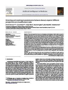
Figure 14: Token distribution for Task 1 ’s DiseaseOutbreaks we can easily compute the degree distribution for the unseen tokens and documents by subtracting the distribution for the retrieved documents from the distribution for the complete database. Next, we report the results of our experimental evaluation of our optimization approaches, to highlight their strengths and weaknesses for choosing execution strategies that reach the target recall τ efficiently.

7

Experimental Setting

We now describe the experimental setting for each text-centric task of Section 2, including the realworld data sets for the experiments. We also present interesting statistics about the task-specific distribution of tokens in the data sets.

7.1

Information Extraction

Document Processor: For this task, we use the Snowball information extraction system [AG00] as the document processor (see Section 3). We use two instantiations of Snowball: one for extracting a DiseaseOutbreaks relation (Task 1a) and one for extracting a Headquarters relation (Task 1b). For Task 1a, the goal is to extract all the tuples of the target relation DiseaseOutbreaks (DiseaseName, Country), which we discussed throughout the article. For Task 1b, the goal is to extract all the tuples of the target relation Headquarters (Organization,Location), where a tuple ho, li in Headquarters indicates that organization o has headquarters in location l. A token for these tasks is a single tuple of the target relation, and a document is a news article from the New York Times archive, which we describe next. Data Set: We use a collection of newspaper articles from The New York Times, published in 1995 (NYT95) and 1996 (NYT96). We use the NYT95 documents for training and the NYT96 documents for evaluation of the alternative execution strategies. The NYT96 database contains 182,531 documents, with 16,921 tokens for Task 1a and 605 tokens for Task 1b. Figures 14 and 15 show the token and document degree distribution (Section 5) for Task 1a: both distributions follow a power-law, a common distribution for information extraction tasks. The distributions are similar

26

Document Degree Distribution 100000

Number of Documents

10000 y = 43060x-3.3863 R2 = 0.9406 1000

100

10

1 1

10 Document Degree

100

Figure 15: Document distribution for Task 1 ’s DiseaseOutbreaks for Task 1b. Execution Plan Instantiation: For Filtered Scan we use a rule-based classifier, created using RIPPER [Coh96]. We train RIPPER using a set of 500 useful documents and 1,500 not useful documents from the NYT95 data set. We also use 2,000 documents from the NYT95 data set as a training set to create the queries required by Automatic Query Generation. Finally, for Iterative Set Expansion, we construct the queries using the conjunction of the attributes of each tuple (e.g., tuple htyphus, Belizei results in query [typhus AND Belize]).

7.2

Content Summary Construction

Document Processor: For this task, the document processor is a simple tokenizer that extracts the words that appear in the eligible documents, defined as a sequence of one or more alphanumeric characters and ignoring capitalization. Data Set: We use the 20 Newsgroups data set from the UCI KDD Archive [BM98]. This data set contains 20,000 messages from 20 Usenet newsgroups. We also randomly retrieve additional Usenet articles to create queries for Automatic Query Generation. Figures 16 and 17 show the token and document degree distribution (Section 5) for this task. The document degree follows a lognormal distribution [Mit04] and the token degree follows, as expected [Zip49], a power-law distribution. Execution Plan Instantiation: For this task, Filtered Scan is not directly applicable, since all documents are “useful.” For Iterative Set Expansion, the queries are constructed using words that appear in previously retrieved documents; this technique corresponds to the Learned Resource Description strategy for vocabulary extraction presented by Callan et al. [CCD99]. Finally, for Automatic Query Generation, we constructed the queries as follows: first, we separate the documents into topics according to the high-level name of the newsgroup (e.g., “comp”, “sci”, and so on); then, we train a rule-based classifier using RIPPER, which creates rules to assign documents into categories (e.g., cpu AND ram → comp means that a document containing the words “cpu” and “ram” is assigned to the “comp” category). The final queries for Automatic Query Generation contain the antecedents of the rules, across all categories. This technique corresponds to the Focused Probing strategy for vocabulary extraction presented by Ipeirotis and Gravano [IG02].

27

Token Degree Distribution 100000

10000

1000

Number of Tokens

100

10

1 1

10

100

1000

10000

100000

Token Degree

Figure 16: Token distribution for Task 2

7.3

Focused Resource Discovery

Document Processor: For this task, the document processor is a multinomial Naive Bayes classifier, which detects the topic of a given web page [CvdBD99]. The topic of choice for our experiments is “Botany.” Data Set: We retrieved 8,000 web pages listed in Open Directory17 under the category “Top → Science → Biology → Botany.” We selected 1,000 out of the 8,000 documents as training documents, and created a multinomial Naive Bayes classifier that decides whether a web page is about Botany. Then, for each of the downloaded Botany pages, we used Google to retrieve all its “backlinks” (i.e., all the web pages that point to that page); again, we classified the retrieved pages and for each page classified as “Botany” we repeated the process of retrieving the backlinks, until none of the backlinks was classified under Botany. This process results in a data set with approximately 12,000 pages about Botany, pointed to by approximately 32,000 useless documents deemed irrelevant to the Botany topic. To augment the data set with additional useless documents, we picked 10 more random topics from the third level of the Open Directory hierarchy and we downloaded all the web pages listed under these topics, for a total of approximately 100,000 pages. After downloading the backlinks for these pages, our data set contained a total of approximately 800,000 pages, out of which 12,000 are relevant to Botany. Execution Plan Instantiation: For this task, the Scan plan corresponds to an unfocused crawl, with a classifier deciding whether each of the retrieved pages belongs to the category of choice. As an instantiation of Filtered Scan, we use the “hard” version of the focused crawler described in [CvdBD99]. The focused crawler starts from a few Botany web pages, and then visits a web page only when at least one of the documents that points to it is useful. Finally, to create queries for Automatic Query Generation, we train a RIPPER classifier using the training set, and create a set of rules that assign documents into the Botany category. We use these rules to query the data set and retrieve documents. 17

http://www.dmoz.org

28

Document Degree Distribution

180 160

Number of Documents

140 120 100 80 60 40 20 0 1

10

100 Document Degree

1000

10000

Figure 17: Document distribution for Task 2

8

Experimental Evaluation

In this section, we present our experimental results. Our experiments focus on the execution times of each alternate execution strategy (Section 4) for the tasks and settings described in Section 7. We compute the actual execution times and compare them against our estimates from Section 5. First, we compute our estimates with exact values for the various parameters on which they rely (e.g., token degree distribution). Then, we measure the execution time using our optimization strategies, which rely on approximate estimates of these parameters, as described in Section 6. Accuracy of Cost Model with Correct Information: The goal of the first set of experiments is to examine whether our cost model of Section 5 captures the real behavior of the alternate execution strategies of Section 4, when all the parameters of the cost model (e.g., token and document degrees, classifier characteristics) are known a-priori. For this, we first measure the actual execution time of the strategies, for varying values of the target recall τ . The lines SC time, FS time, ISE time, AQG time in Figures 18, 19, 20, and 21 show the actual execution time of the respective strategies for the tasks described in Section 7. Then, to predict the execution time of each strategy, we used our equations from Section 5. The lines SC pred, FS pred, ISE pred, AQG pred in Figures 18, 19, 20, and 21 show our execution time estimates for varying values of the target recall τ . The results were exceptionally accurate, confirming the accuracy of our theoretical modeling. The prediction error is typically less than 10% for all values of target recall τ . Furthermore, our modeling captures the characteristics and the limitations of each execution plan. For example, Automatic Query Generation is the fastest execution plan for Task 1a (Figure 18) when the target recall τ is under 0.15. However, due to the limited number of queries generated during the training phase, Automatic Query Generation does not reach higher recall values in our scenario and implementation. (We generated 72 queries for this task.) Our analysis correctly captures this limitation and shows that, for higher recall targets, other strategies are preferable. This limitation also appears for the Iterative Set Expansion strategy, confirming previously reported results [AIG03]. The results are similar for Task 2 and Task 3 : our analysis correctly predicts the execution time and the recall limitations of each strategy. Quality of Choice of Execution Strategies: After confirming that our cost models accu-

29

100,000

10,000

Execution Time (secs)

1,000

100

SC_time

SC_pred

FS_time

FS_pred

ISE_time

ISE_pred

AQG_time

AQG_pred

10 0.00

0.10

0.20

0.30

0.40 0.50 Recall

0.60

0.70

0.80

0.90

1.00

Figure 18: Actual vs. estimated execution times for Task 1a, as a function of the target recall τ rately capture the actual execution time of the alternate execution strategies, we examine whether our optimization strategies lead to the choice of the fastest plan for each value of target recall τ . We start executing each task by using the strategy that is deemed best for the target recall and the available statistics. These statistics are the expected distribution family of the token and document degrees for the task, with some “default” parameters, such as β = 2 for power-law distributions (see Section 7). As we retrieve documents and extract tokens during the actual execution, the available statistics are refined and progressively lead to better estimates of the document and token degree distributions for the complete database. The global optimization approach reconsiders its choice of execution plan every N documents (see Figure 12). For our experiments, we use N = 100, which allows the statistics to change sufficiently between reoptimizations, but —at the same time— without allowing a suboptimal algorithm to run for too long. The local optimization approach defines “combination” executions by picking the best strategy for selecting k tokens at a time (see Figure 13). For our experiments, we set k = 0.05 · |Tokens|. The Global line in Figures 22, 23, 24, and 25 shows the actual execution time, for different recall thresholds, using our global optimization approach. Typically, our global optimizer finishes the task in the same time as the best possible strategy, resulting in execution times that can be up to 10 times faster than alternative plans that we might have picked based on plain intuition or heuristics. For example, consider Task 1b with recall target τ = 0.35 (Figure 23): without our cost modeling, we might select Iterative Set Expansion or Automatic Query Generation, both reasonable choices given the relatively low target recall τ = 0.35. However, Automatic Query Generation cannot achieve a recall of 0.35 and Iterative Set Expansion is more expensive than Filtered Scan for that task. Our optimizer, on the other hand, correctly predicts that Filtered Scan should be the algorithm of choice. In this example, our optimizer initially picked Iterative Set Expansion, but quickly revised its decision and switched to Filtered Scan after gathering statistics from only 1-2% of the database. We should note here that our optimizer’s actual time estimates are often far from the actual execution times, especially at the beginning of the execution when parameter estimates are rough and usually inaccurate. Fortunately, these time estimates are only used to pick the best available strategy, therefore even coarse estimates are sufficient. We observed high time estimation errors frequently in our experiments but, due to the large differences in execution time between the

30

100,000

10,000

Execution Time (secs)

1,000 SC_time FS_time ISE_time AQG_time

100

SC_pred FS_pred ISE_pred AQG_pred

10 0.00

0.10

0.20

0.30

0.40

0.50 Recall

0.60

0.70

0.80

0.90

1.00

Figure 19: Actual vs. estimated execution times for Task 1b, as a function of the target recall τ strategies, our optimizer still managed to pick good execution plans. As the execution progresses, the estimates become increasingly accurate and the optimizer not only identifies the best execution plans but also provides accurate time estimates as well. As another interesting observation derived from out experiments, our prediction algorithm sometimes overestimates the achievable recall of a strategy (e.g., for Automatic Query Generation). In such cases, our (incorrectly picked) strategy runs to completion; then, naturally, our technique picks the “next best” strategy and continues the execution from the point reached by the (incorrectly picked) strategy. In such cases, we sometimes observed a small performance gain derived from this initial mistake, since the “incorrect” strategy outperforms the “correct” strategy for the first part of the execution. This result shows that a multi-strategy execution can often perform better than an optimization strategy that attempts to pick a single execution plan, which is precisely the rationale behind our local optimization approach. The Local line in Figures 26, 27, 28, and 29 shows the actual execution time, for different recall thresholds, using our local optimization approach. Not surprisingly, the local optimizer behaves similarly to the global optimizer for low recall targets, where both optimization approaches proceed similarly. However, the local optimizer becomes noticeably preferable for higher target recall values that are beyond the reach of the fastest execution strategies: the global optimizer, by design, ignores an execution plan if this plan cannot reach the target recall. In contrast, the local optimizer can choose a fast execution strategy for extracting the initial batches of tokens, even if such strategy could not reach the overall target recall; then the local optimizer can pick a slower strategy to continue from the point where the fastest plan has stopped. Interestingly, the advantage of the local optimizer diminishes over time, and its execution times slowly converge towards the execution times of the global optimizer: the local optimizer targets the most promising parts of the database early on, through fast early executions, and the associated speed-ups in the execution diminish as the distribution of tokens over the unseen documents becomes sparser and sparser. Conclusions: We demonstrated how our modeling approach can be used to create an optimizer for text-centric tasks. The presented approach allows for a better understanding of the behavior of query- and crawl-based strategies, in terms of both execution time and recall. Furthermore, our modeling works well even with on-the-fly estimation of the required statistics, and results in

31

1,000.0

Execution Time (secs)

100.0

10.0

SC_pred ISE_pred AQG_pred

1.0

SC_time ISE_time AQG_time

0.1 0.00

0.10

0.20

0.30

0.40

0.50 0.60 Recall

0.70

0.80

0.90

1.00

Figure 20: Actual vs. estimated execution times for Task 2, as a function of the target recall τ close-to-optimal execution times. Our work provides fundamental building blocks towards a full query optimizer for text-centric tasks: given a specific target recall (e.g., “find 40% of all disease outbreaks mentioned in the news”), the query optimizer can automatically select the (combination of) best execution strategies to achieve this recall.

9

Related Work

In this article, we analyzed and estimated the computational costs of text-centric tasks. We concentrated on three important tasks: information extraction (Task 1 ), text database content summary construction (Task 2 ), and focused resource discovery (Task 3 ). Implementations of Task 1 (Section 2.1) traditionally use the Scan strategy of Section 4.1, where every document is processed by the information extraction system (e.g., [Gri97, YG98]). Some systems use the Filtered Scan strategy of Section 4.2, where only the documents that match specific URL patterns (e.g., [Bri98]) or regular expressions (e.g., [GHY02]) are processed further. Agichtein and Gravano [AG03] presented query-based execution strategies for Task 1, corresponding to the Iterative Set Expansion strategy of Section 4.3 and Automatic Query Generation strategy of Section 4.4. More recently, Etzioni et al. [ECD+ 04] used what could be viewed as an instance of Automatic Query Generation to query generic search engines for extracting information from the web. Cafarella and Etzioni [CE05] presented a complementary approach of constructing a specialpurpose index for efficiently retrieving promising text passages for information extraction. Such document (and passage) retrieval improvements can be naturally integrated into our framework. For Task 2, the execution strategy in [CCD99] can be cast as an instance of Iterative Set Expansion, as discussed in Section 4.3. Another strategy for the same task [IG02] can be considered an instance of Automatic Query Generation (Section 4.4). Interestingly, over large crawlable databases, where both query- and crawl-based strategies are possible, query-based strategies have been shown to outperform crawl-based approaches for a related database classification task [GIS02], since small document samples can result in good categorization decisions at a fraction of the processing time required by full database crawls. For Task 3, focused resource discovery systems typically use a variation of Filtered Scan [CvdBD99, 32

1,000,000

100,000

Execution Time (secs)

10,000

1,000

100

SC_time

SC_pred

FS_time

FS_pred

AQG_time

AQG_pred

10 0.00

0.10

0.20

0.30

0.40

0.50 0.60 Recall

0.70

0.80

0.90

1.00

Figure 21: Actual vs. estimated execution times for Task 3, as a function of the target recall τ CPS02,DCL+ 00,MPS04], where a classifier determines which links to follow for subsequent computationally expensive steps of retrieval and processing. Other strategies, which we model as variants of Automatic Query Generation, may also be effective for some scenarios [CS96]. Other important text-centric tasks can be modeled in our framework. One such task is text filtering (i.e., selecting documents in a text database on a particular topic) [Oar97], which can be executed following either Filtered Scan, or, if appropriate, Automatic Query Generation. Another task is the construction of comparative web shopping agents [DEW97]. This task requires identifying appropriate web sites (e.g., by using an instance of Automatic Query Generation) and subsequently extracting product information from a subset of the retrieved pages (e.g., by using an implementation of Filtered Scan). For the task of training named entity recognition systems, Jones [Jon05] showed that named-entity co-occurrence graphs (e.g., involving person and location names) follow a power-law degree distribution, which suggests that the execution of this task might also be modeled in our framework. As another example, web question answering systems [BBDL02] usually translate a natural language question into a set of web search queries to retrieve documents for a subsequent answer extraction step over a subset of the retrieved documents. This process can thus be viewed as a combination of Automatic Query Generation and Filtered Scan. Recently, Ntoulas et al. [NZC05] presented query-based strategies for exhaustively “crawling” a hidden web database while issuing as few queries as possible. Estimating the cost of a query execution plan requires estimating parameters of the cost model. We adapted effective database sampling techniques (e.g., [CMN98, LS95]) for our problem, as we discussed in Section 6. Our work is similar in spirit to query optimization over structured relational databases, adapted to the intrinsic differences of executing text-centric tasks; our work is also related to previous research on optimizing query plans with user-defined predicates [CS99], in that we provide a robust way of estimating costs of complex text-centric “predicates.” Our work can then be regarded as developing specialized, efficient techniques for important special-purpose “operators” (e.g., as was done for fuzzy matching [CGGM03]). Our optimization approach is conceptually related to adaptive query execution techniques developed for relational data. In particular, Ives et al. [IFF+ 99] describe the Tukwila system for distributed processing of joins over autonomous data sources, with no information about table 33

100,000

10,000

Execution Time (secs)

1,000

100

SC_time

FS_time

ISE_time

AQG_time

Global 10 0.00

0.10

0.20

0.30

0.40 0.50 Recall

0.60

0.70

0.80

0.90

1.00

Figure 22: Actual execution times for the four basic execution strategies, as well as for the global optimization approach, for Task 1a and as a function of the target recall τ cardinalities or value distributions and with unpredictable network delays and data arrival rates. Hence any initially chosen execution plan is expected to be adjusted during query execution, as the availability of sources changes or better relevant statistics are obtained. Our optimization approach also revisits the choice of execution strategies for a text-centric task, as documents are retrieved and tokens extracted and, consequently, the statistics on document and token distributions are refined. Our focus in this article is on processing text-centric tasks over a single text “database,” and not on gracefully recovering from unpredictable delays when executing a particular operator in a join pipeline. Our optimization approach is also conceptually related to the eddies work, where a query execution plan is continuously reevaluated after each output tuple [AH00]. The eddies work thus focuses on effective join processing, allowing flexible re-ordering of the query operators. Our optimization approach is also related to the re-optimization methods presented by Kabra and DeWitt [KD98]: the statistics are updated at key points during query execution to re-allocate memory resources for active operators and to potentially adjust the plan for the rest of the execution. The general re-optimization approach of [KD98] for relational data was extended by Markl et al. [MRS+ 04], where the cardinality estimation errors detected during query execution may trigger a re-optimization step for the execution plan. Our general optimization approach behaves similarly, albeit for text-centric tasks, which require different parameter estimation techniques. This article substantially extends our previous work in [AIG03, IAJG06]. Our earlier paper [AIG03] presented preliminary results on modeling and estimating the achievable recall of Iterative Set Expansion, for Task 1 (information extraction) and Task 2 (database content summary construction). Later, in [IAJG06], we developed and evaluated rigorous cost models for Iterative Set Expansion, as well as for three additional general execution strategies, namely Scan, Filtered Scan, and Automatic Query Generation. In [IAJG06], we also presented a principled, cost-based global optimization approach for selecting the most efficient execution strategy automatically. The current article substantially extends the analysis and experimental evaluation in [IAJG06]. In this article, we present a detailed description of our methodology for estimating the parameter values required by our cost model (Sections 6.1.1 through 6.1.4), whereas in [IAJG06], due to space restrictions, we only gave a high-level overview of our techniques. Another substantial new contribution with

34

100,000

Execution Time (secs)

10,000

1,000

SC_time ISE_time Global

100

FS_time AQG_time

10 0.00

0.10

0.20

0.30

0.40

0.50 Recall

0.60

0.70

0.80

0.90

1.00

Figure 23: Actual execution times for the four basic execution strategies, as well as for the global optimization approach, for Task 1b and as a function of the target recall τ respect to [IAJG06] is that now our optimizers do not rely on knowledge of the |Tokens| statistics, but instead estimate this parameter “on-the-fly” as well, during execution of the task. Furthermore, in this article, we present a new, “local” optimizer that potentially builds “multi-strategy” executions by picking the best strategy for each batch of k tokens (Section 6.2). In contrast, the “global” optimization approach in [IAJG06] only attempts to identify a single execution plan that is capable of reaching the full target recall. We implemented the new local optimization approach and compared it experimentally against the global approach of [IAJG06]; the results of the comparison are presented in Figures 26, 27, 28, and 29, in Section 8. The results show the superiority of the local optimizer over the global optimizer. Finally, Jain et al. [JDG07] have very recently presented a query optimization approach for simple SQL queries over (structured data extracted from) text databases. This work heavily relies on information extraction systems and is thus closely related to our Task 1 scenario. Jain et al. [JDG07] consider multiple document retrieval strategies to process a SQL query, including Scan, Automatic Query Generation, and other query-based strategies. Unlike our setting, however, [JDG07] focuses on extraction scenarios that typically involve multiple information extraction systems, whose output might then need to be integrated and joined to answer a given SQL query. The SQL query optimization approach in [JDG07] accounts for errors originating in the information extraction process, and characterizes alternate query executions —which might differ in their choice of extraction systems— based on their precision, as well as on their execution time and recall. An interesting research direction is to incorporate the time and recall estimation models presented in this article into the query processing model of [JDG07].

10

Conclusion

In this article, we introduced a rigorous cost model for several query- and crawl-based execution strategies that underlie the implementation of many text-centric tasks. We complement our model with a principled cost estimation approach. Our analysis helps predict the execution time and output completeness of important query- and crawl-based algorithms, which until now were only 35

1,000.0

Execution Time (secs)

100.0

10.0

1.0

SC_time

ISE_time

AQG_time

Global

0.1 0.00

0.10

0.20

0.30

0.40

0.50 0.60 Recall

0.70

0.80

0.90

1.00

Figure 24: Actual execution times for the three basic execution strategies, as well as for the global optimization approach, for Task 2 and as a function of the target recall τ empirically evaluated, with limited theoretical justification. We demonstrated that our modeling can be successfully used to create optimizers for text-centric tasks, and showed that our optimizers help build efficient execution plans to achieve a target recall, resulting in executions that can be orders of magnitude faster than alternate choices. Our work can be extended in multiple directions. For example, the current framework assumes that the document processors have perfect “precision,” in that they always produce accurate results. Relaxing this assumption and, correspondingly, predicting the precision of the output produced by different strategies is a natural next step. Another interesting direction is to apply our model to other text-centric tasks and also study how to minimize our reliance on task-specific prior knowledge of the token and document distributions for our analysis.

References [AG00]

Eugene Agichtein and Luis Gravano. Snowball: Extracting relations from large plaintext collections. In Proceedings of the Fifth ACM Conference on Digital Libraries (DL 2000), 2000.

[AG03]

Eugene Agichtein and Luis Gravano. Querying text databases for efficient information extraction. In Proceedings of the 19th IEEE International Conference on Data Engineering (ICDE 2003), 2003.

[AH00]

Ron Avnur and Joseph M. Hellerstein. Eddies: Continuously adaptive query processing. In Proceedings of the 2000 ACM SIGMOD International Conference on Management of Data (SIGMOD 2000), pages 261–272, 2000.

[AIG03]

Eugene Agichtein, Panagiotis G. Ipeirotis, and Luis Gravano. Modeling query-based access to text databases. In Proceedings of the Sixth International Workshop on the Web and Databases, WebDB 2003, pages 87–92, 2003.

36

1,000,000

100,000

Execution Time (secs)

10,000

1,000

100

SC_time

FS_time

AQG_time

Global

10 0.00

0.10

0.20

0.30

0.40

0.50 0.60 Recall

0.70

0.80

0.90

1.00

Figure 25: Actual execution times for the three basic execution strategies, as well as for the global optimization approach, for Task 3 and as a function of the target recall τ [BBDL02] Michele Banko, Eric Brill, Susan Dumais, and Jimmy Lin. AskMSR: Question answering using the World Wide Web. In Proceedings of the 2002 AAAI Spring Symposium on Mining Answers from Texts and Knowledge Bases, 2002. [Ber01]

Michael K. Bergman. The Deep Web: Surfacing hidden value. Journal of Electronic Publishing, 7(1), August 2001.

[BM98]

Catherine L. Blake and Christopher John Merz. UCI repository of machine learning databases. http://www.ics.uci.edu/~mlearn/MLRepository.html, 1998.

[Bri98]

Sergey Brin. Extracting patterns and relations from the world wide web. In Proceedings of the First International Workshop on the Web and Databases, WebDB 1998, pages 172–183, 1998.

[CC01]

James P. Callan and Margaret Connell. Query-based sampling of text databases. ACM Transactions on Information Systems, 19(2):97–130, 2001.

[CCD99]

James P. Callan, Margaret Connell, and Aiqun Du. Automatic discovery of language models for text databases. In Proceedings of the 1999 ACM SIGMOD International Conference on Management of Data (SIGMOD’99), pages 479–490, 1999.

[CE05]

Michael J. Cafarella and Oren Etzioni. A search engine for natural language applications. In Proceedings of the 14th International World Wide Web Conference (WWW 2005), pages 442–452, 2005.

[CGGM03] Surajit Chaudhuri, Kris Ganjam, Venkatesh Ganti, and Rajeev Motwani. Robust and efficient fuzzy match for online data cleaning. In Proceedings of the 2003 ACM SIGMOD International Conference on Management of Data (SIGMOD 2003), pages 313–324, 2003. [CL02]

Fan Chung and Linyuan Lu. Connected components in random graphs with given degree sequences. Annals of Combinatorics, 6:125–145, 2002. 37

100,000

10,000

Execution Time (secs)

1,000

Global Local

100

10 0.00

0.10

0.20

0.30

0.40 0.50 Recall

0.60

0.70

0.80

0.90

1.00

Figure 26: Actual execution times for the global and local optimization approaches, for Task 1a and as a function of the target recall τ [CLC95]

James P. Callan, Zhihong Lu, and William Bruce Croft. Searching distributed collections with inference networks. In Proceedings of the 18th Annual International ACM SIGIR Conference on Research and Development in Information Retrieval, SIGIR’95, pages 21–28, 1995.

[CMN98]

Surajit Chaudhuri, Rajeev Motwani, and Vivek R. Narasayya. Random sampling for histogram construction: How much is enough? In Proceedings of the 1998 ACM SIGMOD International Conference on Management of Data (SIGMOD’98), pages 436– 447, 1998.

[Coh96]

William Weston Cohen. Learning trees and rules with set-valued features. In Proceedings of the 13th National Conference on Artificial Intelligence (AAAI-96), Eighth Conference on Innovative Applications of Artificial Intelligence (IAAI-96), pages 709– 716, 1996.

[CPS02]

Soumen Chakrabarti, Kunal Punera, and Mallela Subramanyam. Accelerated focused crawling through online relevance feedback. In Proceedings of the 11th International World Wide Web Conference (WWW11), pages 148–159, 2002.

[CS96]

William Weston Cohen and Yoram Singer. Learning to query the web. In AAAI Workshop on Internet-Based Information Systems, pages 16–25, 1996.

[CS99]

Surajit Chaudhuri and Kyuseok Shim. Optimization of queries with user-defined predicates. ACM Transactions on Database Systems, 24(2):177–228, 1999.

[CvdBD99] Soumen Chakrabarti, Martin van den Berg, and Byron Dom. Focused crawling: A new approach to topic-specific web resource discovery. Computer Networks, 31(11-16):1623– 1640, May 1999.

38

10,000

Execution Time (secs)

1,000

Global

100

Local

10 0.00

0.10

0.20

0.30

0.40

0.50 Recall

0.60

0.70

0.80

0.90

1.00

Figure 27: Actual execution times for the global and local optimization approaches, for Task 1b and as a function of the target recall τ [DCL+ 00]

Michelangelo Diligenti, Frans Coetzee, Steve Lawrence, C. Lee Giles, and Marco Gori. Focused crawling using context graphs. In Proceedings of the 26th International Conference on Very Large Databases (VLDB 2000), pages 527–534, 2000.

[DEW97]

Robert B. Doorenbos, Oren Etzioni, and Daniel S. Weld. A scalable comparisonshopping agent for the world-wide web. In AGENTS ’97: Proceedings of the First International Conference on Autonomous Agents, pages 39–48, 1997.

[DH73]

Richard Oswald Duda and Peter Elliot Hart. Pattern Classification and Scene Analysis. Wiley, 1973.

[ECD+ 04] Oren Etzioni, Michael J. Cafarella, Doug Downey, Stanley Kok, Ana-Maria Popescu, Tal Shaked, Stephen Soderland, Daniel S. Weld, and Alexander Yates. Web-scale information extraction in KnowItAll (preliminary results). In Proceedings of the 13th International World Wide Web Conference (WWW 2004), pages 100–110, 2004. [GGMT99] Luis Gravano, H´ector Garc´ıa-Molina, and Anthony Tomasic. GlOSS: Text-source discovery over the Internet. ACM Transactions on Database Systems, 24(2):229–264, June 1999. [GHY02]

Ralph Grishman, Silja Huttunen, and Roman Yangarber. Information extraction for enhanced access to disease outbreak reports. Journal of Biomedical Informatics, 35(4):236–246, August 2002.

[GIS02]

Luis Gravano, Panagiotis G. Ipeirotis, and Mehran Sahami. Query- vs. crawling-based classification of searchable web databases. IEEE Data Engineering Bulletin, 25(1):43– 50, March 2002.

[Gri97]

Ralph Grishman. Information extraction: Techniques and challenges. In Information Extraction: A Multidisciplinary Approach to an Emerging Information Technology, International Summer School, (SCIE-97), pages 10–27, 1997. 39

1,000.0

Execution Time (secs)

100.0

10.0

Global

1.0

Local

0.1 0.00

0.10

0.20

0.30

0.40

0.50 0.60 Recall

0.70

0.80

0.90

1.00

Figure 28: Actual execution times for the global and local optimization approaches, for Task 2 and as a function of the target recall τ [IAJG06]

Panagiotis G. Ipeirotis, Eugene Agichtein, Pranay Jain, and Luis Gravano. To search or to crawl? Towards a query optimizer for text-centric tasks. In Proceedings of the 2006 ACM SIGMOD International Conference on Management of Data (SIGMOD 2006), pages 265–276, 2006.

[IFF+ 99]

Zachary G. Ives, Daniela Florescu, Marc Friedman, Alon Y. Levy, and Daniel S. Weld. An adaptive query execution system for data integration. In Proceedings of the 1999 ACM SIGMOD International Conference on Management of Data (SIGMOD’99), pages 299–310, 1999.

[IG02]

Panagiotis G. Ipeirotis and Luis Gravano. Distributed search over the hidden web: Hierarchical database sampling and selection. In Proceedings of the 28th International Conference on Very Large Databases (VLDB 2002), pages 394–405, 2002.

[JDG07]

Alpa Jain, AnHai Doan, and Luis Gravano. SQL queries over unstructured text databases (poster paper). In Proceedings of the 23rd IEEE International Conference on Data Engineering (ICDE 2007), 2007. To appear.

[Jon05]

Rosie Jones. Learning to Extract Entities from Labeled and Unlabeled Text. PhD thesis, Carnegie Mellon University, School of Computer Science, 2005.

[KD98]

Navin Kabra and David J. DeWitt. Efficient mid-query re-optimization of sub-optimal query execution plans. In Proceedings of the 1998 ACM SIGMOD International Conference on Management of Data (SIGMOD’98), pages 106–117, 1998.

[LS95]

Yibei Ling and Wei Sun. An evaluation of sampling-based size estimation methods for selections in database systems. In Proceedings of the 11th IEEE International Conference on Data Engineering (ICDE 1995), pages 532–539, 1995.

[Mit04]

Michael Mitzenmacher. Dynamic models for file sizes and double pareto distributions. Internet Mathematics, 1(3):305–334, 2004. 40

1,000,000

100,000

Execution Time (secs)

10,000

1,000 Global

100

Local

10 0.00

0.10

0.20

0.30

0.40

0.50 0.60 Recall

0.70

0.80

0.90

1.00

Figure 29: Actual execution times for the global and local optimization approaches, for Task 3 and as a function of the target recall τ [MPS04]

Filippo Menczer, Gautam Pant, and Padmini Srinivasan. Topical web crawlers: Evaluating adaptive algorithms. ACM Transactions on Internet Technology, 4(4):378–419, November 2004.

[MRS+ 04] Volker Markl, Vijayshankar Raman, David Simmen, Guy Lohman, Hamid Pirahesh, and Miso Cilimdzic. Robust query processing through progressive optimization. In Proceedings of the 2004 ACM SIGMOD International Conference on Management of Data (SIGMOD 2004), pages 659–670, 2004. [NSW01]

Mark E. J. Newman, Steven H. Strogatz, and Duncan J. Watts. Random graphs with arbitrary degree distributions and their applications. Physical Review E (Statistical, Nonlinear, and Soft Matter Physics), 64(2):026118 (1–17), August 2001.

[NZC05]

Alexandros Ntoulas, Petros Zerfos, and Junghoo Cho. Downloading textual hidden web content by keyword queries. In Proceedings of the Fifth ACM+IEEE Joint Conference on Digital Libraries (JCDL 2005), 2005.

[Oar97]

Douglas W. Oard. The state of the art in text filtering. User Modeling and UserAdapted Interaction, 7(3):141–178, 1997.

[Ros02]

Sheldon M. Ross. Introduction to Probability Models. Academic Press, 8th edition, December 2002.

[SAC+ 79]

Patricia G. Selinger, Morton M. Astrahan, Donald D. Chamberlin, Raymond A. Lorie, and Thomas G. Price. Access path selection in a relational database management system. In Proceedings of the 1979 ACM SIGMOD International Conference on Management of Data (SIGMOD’79), pages 23–34, 1979.

[Seb02]

Fabrizio Sebastiani. Machine learning in automated text categorization. ACM Computing Surveys, 34(1):1–47, March 2002.

41

[Vap98]

Vladimir Naumovich Vapnik. Statistical Learning Theory. Wiley-Interscience, September 1998.

[Wil90]

Herbert S. Wilf. Generatingfunctionology. Academic Press Professional, Inc., 1990.

[YG98]

Roman Yangarber and Ralph Grishman. NYU: Description of the Proteus/PET system as used for MUC-7. In Proceedings of the Seventh Message Understanding Conference (MUC-7), 1998.

[Zip49]

George Kingsley Zipf. Human Behavior and the Principle of Least Effort. AddisonWesley, 1949.

42