Building a MATLAB Graphical User Interface to Solve ... - Shodor

Journal of Computational Science Education

Volume 9, Issue 1

Building a MATLAB Graphical User Interface to Solve Ordinary Di�erential Equations as a Final Project for an Interdisciplinary Elective Course on Numerical Computing Steve M. Ruggiero∗

School of Chemical Engineering Oklahoma State University Stillwater, OK

Jianan Zhao∗

School of Chemical Engineering Oklahoma State University Stillwater, OK

ABSTRACT A �nal project assignment is described for an interdisciplinary applied numerical computing upper division and graduate elective in which students develop a GUI for de�ning and solving a system of ordinary di�erential equations (ODEs) and the associated explicit algebraic equations such as values for parameters. The primary task is to use the MATLAB built-in graphical user interface development environment (GUIDE) [16, 17] to develop a graphical user interface (GUI) that takes a user-speci�ed number of ODEs and explicit algebraic equations as input, solves the system of ODEs using ode45, returns the solution vector, and plots the solution vector components vs. the independent variable. The code for the GUI must be veri�ed by showing that it returns the same results and the same �gures as a system of ODEs with a known solution. The purpose of the �nal project assignment is threefold: (1) to practice GUI design and construction in MATLAB, (2) to verify code implementation, and (3) to review content covered throughout the course. The manuscript �rst introduces the course and the context and motivation for the project. Then the project assignment is detailed. Two student project submissions are described. The veri�cation case study is also provided.

KEYWORDS numerical methods, graduate education, computational science elective course

1

INTRODUCTION

The corresponding author of this paper teaches a course titled Applied Numerical Computing for Scientists and Engineers that she developed at Oklahoma State University. The course is o�ered as a chemical engineering upper division and graduate elective designed and advertised to be interdisciplinary. Over the �rst two o�erings, �ve chemical engineering seniors took the course along with the ∗ The

�rst two authors contributed equally to this work. author.

† Corresponding

Permission to make digital or hard copies of all or part of this work for personal or classroom use is granted without fee provided that copies are not made or distributed for pro�t or commercial advantage and that copies bear this notice and the full citation on the �rst page. To copy otherwise, or republish, to post on servers or to redistribute to lists, requires prior speci�c permission and/or a fee. Copyright ©JOCSE, a supported publication of the Shodor Education Foundation Inc. © 2018 JOCSE, a supported publication of the Shodor Education Foundation Inc. DOI: https://doi.org/10.22369/issn.2153-4136/9/1/4

May 2018

Ashlee N. Ford Versypt†

School of Chemical Engineering Oklahoma State University Stillwater, OK [email protected]

following numbers of graduate students by degree program: eight in chemical engineering, six in mechanical engineering, two in chemistry, and one each in environmental engineering, mathematics, and plant and soil sciences. The �rst and second authors of this paper took the course as �rst year chemical engineering graduate students in the �rst and second course o�erings, respectively. The course is designed to train science and engineering seniors and graduate students to use practical software tools for computational problem solving and research: Git for version control, LATEX for mathematical and scienti�c typesetting, and MATLAB and Python as high level programming languages with libraries of solvers, visualization tools, and capabilities for designing graphical user interfaces (GUIs). Throughout the course, the instructor emphasizes best practices of open-source code development, veri�cation, and documentation [2, 3, 8–15, 18, 20–23, 26, 28] and adopts the Software Carpentry philosophy of providing hands-on training in very practical computational skills for scientists and engineers [27]. Rather than covering the basics of computer programming or details of algorithms for numerical methods, the course focuses on applying numerical computing methodologies, primarily ordinary di�erential equation solvers and optimization routines for parameter estimation to solve realistic continuum scale problems in science and engineering. The course consists of ten reading assignments worth 2% each and six computational assignments. The �rst assignment is worth 5% and introduces the students to using version control in Git and document typesetting in LATEX, which are required components in all subsequent assignments. The second assignment is worth 5% and gives student practice with programming in MATLAB while developing best practices for scienti�c computing. The students are required to create a function de�ning a system of ordinary di�erential equations (ODEs) and write well-documented code. The third assignment is worth 10% and involves using built-in functions and library routines for numerical methods (speci�cally ODE solvers) in MATLAB and Python to solve the system of ODEs described in Appendix A. The fourth assignment is worth 15% and covers parameter estimation of dynamic models using MATLAB and Python focusing on a case study from [1]. The �fth assignment is worth 15% and involves creating a relatively straightforward GUI in MATLAB to take user inputs and display simulation results from user-de�ned functions provided by the instructor for di�erent scienti�c applications. The sixth and �nal computational assignment is worth 30% of the course grade and is described in detail in this paper.

ISSN 2153-4136

19

Volume 9, Issue 1

Journal of Computational Science Education

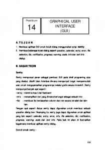
The �nal computational assignment is referred to as the “�nal project” to emphasize its signi�cance in the course grade, its comprehensive nature, and the time involved to complete the assignment satisfactorily. The students are allowed one month to work on this project, and it serves as a take-home �nal exam. The purpose of this assignment is threefold: (1) to practice GUI design and construction in MATLAB, (2) to verify code implementation, and (3) to review content covered throughout the course. The project builds upon content from all of the previous assignments. Although it does not explicitly involve parameter estimation, the systems of ODEs used for the dynamic models in the fourth assignment from [1] are used in the �nal project as two of the three veri�cation cases required. For brevity we only provide the most complicated of the veri�cation cases here in Appendix A, which is from the third assignment. In the chemical reaction engineering course that the corresponding author teaches and many other o�erings of the same course around the U.S., the software POLYMATH [25] is used as recommended by the popular textbook [4], which uses the software throughout the book in many examples and homework problems. POLYMATH is a numerical computation package that can solve data regressions and systems of simultaneous ODEs, linear algebraic equations, or nonlinear algebraic equations. These are all of the types of computational science problems encountered in a typical chemical reaction engineering course. In POLYMATH, equations are entered through GUIs in formats that look just like the written form of the equations, so there is not a coding learning curve (Fig. 1 and Fig. 2). After entering equations via GUIs or in lieu of using the GUIs, users can edit code directly in a script �le. For details on how to use POLYMATH to enter and solve a system of ODEs, a tutorial document is available on the web [5]. A limitation of the current POLYMATH educational version is that users can enter only 30 simultaneous ODEs and 40 explicit algebraic equations. This is adequate for typical use. However, for the course project in the author’s chemical reaction engineering course [6], the limit is often reached. Additionally, POLYMATH cannot combine di�erent types of numerical solvers in the same problem unlike other software programs such as MATLAB and Python. The author originally started programming MATLAB or Python scripts for working around the equation number limit in POLYMATH but found the codes to be challenging for novice users to modify. The �nal project discussed here grew out of a need to have a POLYMATH-like GUIbased platform built into a more sophisticated software platform when dealing with more than 30 simultaneous ODEs. MATLAB was selected for this �nal project because of its relative ease in creating GUIs and packaging them as apps, which are very user-friendly for download and installation. The remainder of this paper provides the required tasks in the �nal project assignment in Section 2, gives details of two student project submissions in Section 3, and o�ers conclusions in Section 4. The veri�cation case study is presented in Appendix A.

2

PROJECT ASSIGNMENT

In the project assignment, students develop a GUI for de�ning and solving a system of ODEs and the associated explicit algebraic equations (e.g., temperature dependence of rate constants or values for parameters) for di�erent applications. The primary task is to

20

Figure 1: Graphical user interface in POLYMATH for entering a di�erential equation.

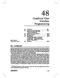
Figure 2: Graphical user interface in POLYMATH for entering an explicit algebraic equation. use the MATLAB built-in graphical user interface development environment (GUIDE) to develop a graphical user interface (GUI) that takes a user-speci�ed number of di�erential equations and explicit algebraic equations as input, solves the system of ODEs using ode45, returns the solution vector, and plots the solution vector components vs. the independent variable. The GUI should work in general for any system of ODEs (speci�cally initial value problems not boundary value problems). The code for the GUI must be veri�ed by showing that it returns the same results and the same �gures as the systems of ODEs de�ned in Computational Assignments 3 and 4. The more complicated of these veri�cation cases is provided in detail in Appendix A. Students are not penalized if their code does not work for arbitrary ODEs beyond the veri�cation cases. The GUI can take a variety of layouts, which may involve use of multiple .m �les, if desired. A descriptive �le naming system should be used. Students should design a GUI that is intuitive to use with the following required as buttons: • de�ne a system of ODEs – The numbers of di�erential equations and algebraic equations should be solicited either directly or indirectly.

ISSN 2153-4136

May 2018

Journal of Computational Science Education

•

•

•

•

Volume 9, Issue 1

⇤ In the direct method, when this button is clicked, a window should appear asking the user how many equations of both types that they want to de�ne. After that windows should appear recursively for the user to enter the speci�ed numbers of corresponding di�erential equations and algebraic equations. ⇤ In the indirect method, when this button is clicked, windows should be opened for de�ning di�erential or algebraic equations one at a time (or in bulk for algebraic equations). At the end of each input, the user chooses done or continue to enter another equation of the same type. The number of equations of that type is then incremented. – The interfaces for entering the equations should be similar to those used in POLYMATH (Figs. 1 and 2), which can be implemented using one or more windows that are themselves GUIs and/or dialog boxes. – The user must be able to enter initial values and limits of integration. – The comment section and the buttons labeled Clear and Cancel shown in the POLYMATH examples (Figs. 1 and 2) are optional. – After input is provided by the user, it should be visible to them as a static textbox, editable textbox, or listbox with options to edit the input. calculate results – This button should calculate results in preparation for either exporting to Excel or plotting. – Something should be output to indicate that the results were calculated; command window output is acceptable. plot results The plot routine should have options for displaying all or a subset of the output vectors (dependent variables vs. the independent variable). save plot – The save plot button should call export_fig.m [19] to create a .png �le of a reasonable size for the output plot that currently appears on the screen. – The user should be prompted to specify a �lename and target directory for the plot. – A sample callback function for a button that saves a plot with a prescribed name via export_fig.m is shown in Fig. 3. export results as Excel �le The export results button should export all the independent and dependent variable output from the ODE solver to a .csv or .xls or .xlsx �le (label the type of output on your GUI) so that the user could view the results in Excel for creating more elaborate plots.

Additional buttons or other GUI objects may be useful. For example, a .mat �le is recommended for saving selected variables from a subsidiary GUI window for de�ning the ODEs or the explicit equations. Then this can be loaded in the main GUI �le to read the values after the temporary GUI window closes. A cell array is a natural way to save the values generated from each of the GUI

May 2018

1 2 3 4 5 6 7 8 9

10 11 12 13 14 15 16

17 18

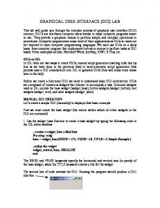
% Executes on button press in saveplot_button function saveplot_button_Callback(hObject, ... eventdata, handles) % hObject handle to saveplot_button % eventdata reserved % handles structure with handles and user data if exist('plotName.png', 'file') == 2 beep h = msgbox(... 'plotName.png already exists. Please rename ... or delete the existing plotName.png file ... before trying to save again.',... 'Plot NOT Saved'); else ax = handles.plotAxes; figure_handle = isolate_axes(ax); export_fig plotName.png h = msgbox(... 'The plot was successfully saved as ... plotName.png. Be careful to rename it if ... you want to save multiple versions of ... the plot.',... 'Plot Saved'); end

Figure 3: saveplot_button_Callback function example. windows; however, other ways are acceptable. Another useful button could allow users to edit the axes labels, particularly to include units. The GUI must be packaged as a MATLAB app and submitted electronically via the course website. Students must create a .tex �le to document testing that their GUI works for the veri�cation test cases. A screenshot of the GUI when all equations have been entered must be included as well as the output plot with all of the dependent variables plotted together vs. the independent variable. A veri�cation case is described further in Appendix A. String manipulation is not the primary purpose of the �nal project, but it is necessary to take input from di�erent windows and compose strings into equations. To aid students less familiar with string manipulation, the following tips are provided. If the code can accept the proper input arranged as cell arrays, the function shown in Fig. 4 connects the input to the ODE solver. In test cases, it is clear that the numerator and denominator are not exactly the strings that are needed for ode45(@(t,y)ODE...) and that the explicit equations and the right hand sides of the ODEs are not in terms of and t as desired. It is strongly advised NOT to use strrep in MATLAB or other �nd and replace algorithms. Instead, let MATLAB do that automatically by parsing the strings. Fig. 4 is a working version of a function ODE that properly reads cell array inputs stored as variables in handles and converts them to the equations that de�ne the system of ODEs. ODE is called by ode45. The only requirement to the user is that they cannot name a constant parameter or t. This requirement is not necessary for independent or dependent variables.

3

STUDENT PROJECT SUBMISSIONS

The top student submissions for the �nal project from each of the �rst two course o�erings are presented here as examples. We have prepared a private Bitbucket version control repository for

ISSN 2153-4136

21

Volume 9, Issue 1

1 2 3 4 5 6 7 8 9 10 11 12 13 14 15 16 17

Journal of Computational Science Education

function dydt = ODE(t, y, denominators, ... numerators, RHSs, explicitEqns) % Input: t and y are the independent and % dependent variable values, % denominators, numerators, RHSs, and % explicitEqns are cell arrays with % the first three terms defining the % ODEs of the form˘ a % d(numerators) / d(denominators) = RHSs % and the fourth term defining the associated % explicit equations % Output: the derivative vector dy/dt for % y(1):y(numODEs) where % numODEs = length(numerators) = length(RHSs) = length(denominators) % To be called by ode45(@(t,y)... % ODE(t,y,denominators,numerators,RHSs,... % explicitEqns), tspan, y0)

18 19 20 21 22 23 24 25 26 27 28 29 30 31 32 33 34 35 36 37 38 39 40

% independent variable str0=cell2mat(denominators(1)); eval(strcat(str0,'=t;')); % dependent variables for i = 1:length(numerators) str1 = cell2mat(numerators(i)); eval(strcat(str1,'=y(i);')); end % explicit equations provided in MATLAB % acceptable order; can be a % semicolon separated list for i = 1:length(explicitEqns) str2 = cell2mat(explicitEqns(i)); eval(str2); end % Right-hand sides of ODE definitions for i = 1:length(RHSs) str3 = cell2mat(RHSs(i)); dydt(i) = eval(str3); end % output formatting dydt = dydt';

Figure 4: Example ODE function that properly reads cell array inputs stored as variables in handles and converts them to the equations that de�ne the system of ODEs. archiving the code for these submissions along with the instructor documents related to the project assignment. The link is not shared publicly here to prevent future students from simply downloading the solution without doing the project. Interested educators may contact the corresponding author by email to request access to the private repository.

3.1

Submission 1

3.1.1 Overview. The program of Submission 1 is mainly composed of three parts: collecting user inputs to de�ne the system of ODEs and the explicit equations, solving the system of ODEs coupled to the explicit equations, and saving simulation results by exporting calculated values and �gures of plots. 3.1.2 GUI Description. The main GUI is composed of ten push buttons, three listboxes, and one axes (plot) object (Fig. 5). The user can provide inputs through the push buttons. List boxes are used to display the ODEs, corresponding initial conditions, and the explicit equations. The axes object is used to display plots of some or all of the dependent variables as functions of the independent variable

22

(Fig. 5 shows only the �rst dependent variable selected). Multiple GUI windows are used for this program. All the push buttons, except Reset and Help, were separated into three groups based on the objectives of the program. Within the panel labeled Define/Edit Equations/Parameters, the Define Equations push button �rst allows the user to specify the number of ODEs and gives the user an option to choose whether or not to de�ne any explicit equations after the system of ODEs is de�ned (Fig. 6). If the radio button Add explicit equations is activated (Fig. 6), a GUI window appears that allows user to enter the explicit equations in bulk (Fig. 7) after the system of ODEs has been successfully de�ned. All the ODEs must have explicit form d of dt = f (t, ). Based on the input number of ODEs, a for loop is used to repeatedly pop up the window for de�ning each ODE separately along with its initial value (Fig. 8). When the loop is �nished, a new GUI window lets the user de�ne the upper and lower limits of the integration, with both having default values of 0 (Fig. 9). The speci�ed values and equations all appear in the main GUI window either in listboxes or as static text (Fig. 5). The remaining buttons in the �rst panel in Fig. 5 are used for editing. The Edit Selected ODE push button enables the user to edit speci�c ODE expressions and the corresponding initial value according to selected line in the ODE(s)Entered list box (Fig. 5). By clicking the Integration Limits push button, the user can modify the integration limits via the dialog box (Fig. 9). Through the Edit Explicit Eqs push button, the user opens a new GUI window (Fig. 7) to de�ne the explicit equations if they have not been de�ned yet or to edit existing explicit equations. In the Calculate/Plot panel, clicking the push button Calculate opens a dialog window to require the user to enter the step size for the numerical integration. The default value is 10 4 . Then ode45 is called to solve the system of ODEs. When the Plot Results button is pushed, the window titled Select Variables Shown on Plot appears to allow the user to select single or multiple dependent variables to be shown on the axes of the main GUI (Fig. 10). The user can modify the labels of the independent and dependent axes via the push button Edit Plot Axes. The default axes labels are shown in Fig. 11. The Save Plot push button enables the user to specify a �le name and target local directory for saving the plot currently shown in the axes area of the main GUI. Similarly, the Save Data to .csv push button prompts the user to provide a �le name and local directory for saving all the results for the independent and dependent variable output from the ODE solver to a .csv �le. The program is capable to some extent of checking for the legality of user inputs. In the window to de�ne a di�erential equation (Fig. 8), the numerator and denominator positions are checked for the presence of characters and the initial condition blank is checked for a numerical value. The upper limit of integration is required to be larger than the lower limit. When the user decides to edit the notation of the independent variable, the program can only change the left hand side of every ODE; therefore, the user needs to make sure the notation is also modi�ed on the right hand side of each ODE to avoid any errors during the calculation. 3.1.3 Program Verification. We entered the system of equations from Appendix A into the program, calculated the results, and

ISSN 2153-4136

May 2018

Journal of Computational Science Education

Volume 9, Issue 1

Figure 5: Submission 1 main GUI screenshot with plot of the dependent variable T for the veri�cation case in Appendix A.

Figure 6: Submission 1 dialog box for setup of the number of equations.

plotted two di�erent sets of the dependent variables in Figs. 5 and 12 to see the curves clearly on their di�erent scales. 3.1.4 Program Shortcomings. One major defect of this program is that after the number of ODEs is de�ned at the very beginning, it cannot be changed unless the user rede�nes the whole system of equations. This program did not utilize the MATLAB GUI handles structure for passing arguments between functions. The de�ciency related to not being able to edit the number of equations could be compensated by adding another function to manipulate the master ode_eqs.mat �le, which stores the expressions for all the equations. This could be modi�ed carefully by adding another ODE or deleting one or several existing ODEs. Alternatively, the program

May 2018

Figure 7: Submission 1 dialog box to enter the explicit equations.

could be restructured to utilize the handles, in which case an update to the number of ODEs would not be as tricky to implement. Another defect is that the program is not capable of accepting explicit equations in arbitrary order as in POLYMATH, meaning that a parameter in an explicit equation must be de�ned before it is used. This requires extra work from the users as all the explicit equations have to be listed in a certain order. This is how MATLAB reads codes, so this is not a serious problem. For possible solutions to this problem, see Submission 2 presented in Section 3.2.

ISSN 2153-4136

23

Volume 9, Issue 1

Journal of Computational Science Education

Figure 11: Submission 1 dialog box to edit axes labels starting from default axes labels.

Figure 8: Submission 1 dialog box to enter a di�erential equation.

Figure 9: Submission 1 dialog box to de�ne limits of integration. Figure 12: Submission 1 plots of the dependent variables F A , F B , and FC for the veri�cation case in Appendix A. When the user modi�es an ODE, only one ODE from the list box can be selected at one time. Also, items in the Initial Value(s) list box can be selected; however, they are not related to any push buttons. In a future version, a new GUI could be added to allow the user to edit initial values based on the selected line in the Initial Value(s) list box independent of editing the corresponding ODE.

3.2

Figure 10: Submission 1 dialog box to select which variables to display on the plot.

24

Submission 2

3.2.1 Overview. Submission 2 goes beyond the scope of the project requirements by allowing the user the capability to freely edit equations in the GUI and to enter equations in any order (Fig. 13). Allowing the text to be edited enables the user to wholesale copy text in order to share, save, and enter equations. Additionally, if an error is made in entering the equations into the dialog boxes, the user can quickly �x it by editing the text directly. Furthermore, if the user is comfortable, they can type their equations directly without using the dialog boxes. This is very consistent with the capabilities of POLYMATH.

ISSN 2153-4136

May 2018

Journal of Computational Science Education

Volume 9, Issue 1

Figure 13: Submission 2 main GUI screenshot.

Figure 14: Submission 2 dialog box for entering ODEs. 3.2.2 GUI Description. The main GUI is composed of one editable textbox, six push buttons, and one axes (plot) object (Fig. 13). The user can provide inputs through the push buttons in much the same manner as in Section 3.1 through a GUI for de�ning a di�erential equation (Fig. 14) and a GUI for de�ning a single explicit algebraic equation (Fig. 15). The axes object is used to display plots of some or all of the dependent variables as functions of the independent variable (Fig. 13 shows all of the dependent variables selected). The editable textbox is described in detail in the remainder of this section. 3.2.3 Equation Parsing. Properly supporting an editable textbox for equation entry presents some key issues. If the text displayed in the app cannot be edited, then input can be gathered solely from dialog boxes in a very structured manner such as in Section 3.1. Since an editable textbox is a much less structured form of input, interpreting the input becomes a major challenge. The �rst step in handling the input is to parse the text and convert the text into

May 2018

Figure 15: Submission 2 dialog box for entering algebraic equations. a structured format. The second step is to reorder the equations so that each equation is only dependent on either no equations or only previously de�ned equations. This is a requirement because MATLAB requires a variable to be de�ned before it can be used. The GUI does have dialog boxes that can be used to enter equations (Figs. 14–15); however, these dialog boxes do little more than formatting and inserting the appropriate text into the editable textbox as a template for the user to see how to edit the text. To parse the text entered into the textbox of the GUI, a custom function ParseEq.m accepts a string as an argument and returns a cell array that contains 4 elements. The four elements are the name of the variable the equation solves for, the independent variable associated with the equation if the equation is an ODE, a structure containing the results of parsing the right hand side of the equation, and the type of equation. The right hand side of the equation is returned in two parts: a string of code that can be executed to solve for the dependent variable and a list of variables that need to be de�ned before the code can be evaluated.

ISSN 2153-4136

25

Volume 9, Issue 1

Journal of Computational Science Education

At the heart of parsing the entered text is the use of regular expressions. Regular expressions are useful for �nding speci�c sequences of text. Regular expressions make use of wildcards, whitespace characters, alphanumeric ranges, and more to create a very powerful and �exible syntax for matching text. For example, in the GUI the left hand side of an ODE is in the form of d(y)/d(t), where and t can be any variables. The regular expression ‘d\(\w*\)\/d\( \w*\)’ will match the left hand side of any correctly entered ODE. The �rst step in parsing the equations is to break the equation into two parts for the left- and right-hand sides. This is done by searching for the ‘=’ character and taking either side as separate strings. Of the two sides, the left-hand side is evaluated �rst. The left-hand side of each equations has a speci�c structure–the exact form depends on if the equation is an algebraic equation, ODE, an initial value, or the range of an independent variable. The structured left-hand side of each equation lends itself to being easily parsed through regular expressions. The main concept used in parsing the right-hand side of an equation is to build a line of code by following order of operations to identify the calculation to be done �rst, producing the code to evaluate the operation, and then abstracting the evaluated term from the rest of the equation using a token. For example, the string `x + y * z' becomes `x + #1', where #1 is placeholder for a structure containing the results of parsing `y * z'. Parsing the right-hand side becomes more complex when handling parentheses. The approach to handling parentheses is to replace the portion of the equation inside of the parenthesis with a token and then recursively calling theParseEq.m function with the replaced text. The result is that for each nested level of parentheses, the function is recursively called until the innermost level of parentheses is reached and evaluated normally. 3.2.4 Equation Reordering. The problem of ordering the equations is reduced to a problem similar to Gaussian elimination. A matrix is constructed where each row represents a dependent variable, and each column represents a unique variable needed to de�ne a variable. For each dependent variable, the element in the column of each variable needed to de�ne the dependent variable is set to 1. For example, the equations x =2

(1)

= 3⇤x

(2)

z = 4⇤ +x

(3)

yield the matrix (with columns and rows labeled for clarity) x y z

x 0 1 1

y 0 0 1

4

CONCLUSIONS

The project assignment has been used for 21 total students across two o�erings of the Applied Numerical Computing elective course at Oklahoma State University. The project has been challenging and thought provoking for the students in the course without being unreasonable and overly time-consuming. Each student has typically visited the instructor’s o�ce hours more than once over the one month time period allotted for the project. The instructor has o�ered assistance with debugging and brainstorming and implementing approaches. The most challenging aspect of the project for most students is connecting the input from a subsidiary GUI window back to the main GUI window. The submissions described here provide two di�erent methods for doing this, and the instructions and tips from the instructor in the assignment and in Fig. 4 suggest another alternative using .mat �les and cell arrays. Students are encouraged to discuss ideas with their classmates, but the project must be an individual e�ort. The vast majority of the students have earned an A on the project (all who started early enough to complete all of the required components, including the veri�cation cases). The students have given the project a positive reception as they can clearly see how it connects the prior course content related to numerical solution of systems of ODEs and development of GUIs for scienti�c applications. The project detailed in this paper can be easily integrated into a variety of computational science and engineering elective or required courses. The content is approachable for both senior undergraduates and graduate students from a variety of disciplines given su�cient background in MATLAB programming and GUI design. Additional cases studies could be used to adapt the project to other disciplines such as numerical methods, computational physics or chemistry, mathematical biology, and other �elds of engineering. These case studies could readily be developed from textbook examples in these �elds or published modeling studies such as [1] in petrochemical manufacturing, [7] in computational pharmacology, and [24] in mathematical biology.

A

Each dependent variable that is de�ned by an ODE has an associated initial value previously de�ned. Therefore, all of the columns associated with variables de�ned in ODEs are zeroed out right after creating the matrix, representing the fact that the variable is de�ned. Each dependent variable has exactly one equation in which the variable will show up on the left hand side. When a row corresponding to a variable is zeroed out, the associated equation

26

is put at the bottom of the list of equations, and the column associated with the variable is zeroed out. This process repeats until no changes occur in the matrix after an iteration. If the matrix is not completely zeroed out, then any rows that are not entirely zeros represent variables that are not properly de�ned, and an error is returned to the user containing the variables that are improperly de�ned. If the entire matrix is zeroed out, then the list of equations recorded while zeroing out the matrix is the correct order for the equations so that each equation is only dependent on the previous equation.

VERIFICATION CASE

For the veri�cation case study, a system of ODEs is used as de�ned and solved in an example in a chemical reaction engineering textbook [4]. The equations describe the mass and energy balances for a pair of gas-phase reactions that occur in a plug �ow reactor that is operated non-isothermally:

ISSN 2153-4136

A 2A

k1

!B

k2

!C

(4)

r 1A = k 1AC A 2 r 2A = k 2AC A

(5)

May 2018

Journal of Computational Science Education

Volume 9, Issue 1

where A, B, and C are chemical species, r i j is the reaction rate of the ith reaction with respect to the jth species, and ki j is the kinetic rate constant for the ith reaction with respect to the jth species. Pure A is fed at a rate of 100 mol/s, a temperature of 423 K, and a concentration of 0.1 mol/L. The molar �ow rates of each species, F A , F B , and FC , and the temperature, T , as functions of the reactor volume, V , are the quantities of interest. Mole balances on each species A, B, and C give the ODEs dF A = rA (6) dV dF B = rB (7) dV dFC = rC (8) dV where r i is the net reaction rate of species i. The initial conditions are F A (0) = 100 mol/s, F B (0) = 0 mol/s, FC (0) = 0 mol/s, and T (0) = 423 K. The corresponding elementary rate laws that describe reactions 1 and 2 from (4) and (5), respectively, are (9)

r 1A = k 1AC A 2 k 2AC A

r 2A = (10) where C A is the concentration of species A. The relative rates are r 1B = r 1A = k 1AC A k 2A 2 1 r 2C = r 2A = C 2 2 A Equations (9)–(12) are combined to yield the net rates, r A = r 1A + r 2A = k 1AC A

2 k 2AC A

(11) (12) (13)

r B = r 1B = k 1AC A (14) k 2A 2 rC = r 2C = C (15) 2 A The gas-phase stoichiometry without pressure drop is used to de�ne the concentration of species A as C A = CT (0)

F A T (0) FT T where the total �ow rate is de�ned by

(16)

FT = F A + F B + FC

(17)

The rate constants depend on the temperature through the following Arrhenius functions:  ✓ ◆ E1 1 1 k 1A = 10 exp s 1 (18) R T (0) T  ✓ ◆ E2 1 1 L k 2A = 0.09 exp (19) R T (0) T mol · s The energy balance for the reactor is dT U a(Ta T ) + r 1A H Rx 1A + r 2A H Rx 2A = dV F AC P A + F B C P B + F C C P C

(20)

The values for the remaining parameters representing physical constants are listed in Table 1. To summarize, the system of ODEs for the veri�cation case is F A d F B d FC dT , describing given by (6)–(8) and (20) for ddV , dV , dV , and dV the molar �ow rates of species, A, B, and C, in mol/s and temperature, T , in K in a non-isothermal plug �ow reactor. The reactions

May 2018

Table 1: Values of parameters for the veri�cation case study. Variable

Value

Units

E 1 /R E 2 /R CT (0) H Rx 1A H Rx 2A C PA CPB C PC Ua Ta

4000 9000 0.1 -20,000 -60,000 90 90 180 4000 373

K K mol/L J/(mol of A reacted in reaction 1) J/(mol of A reacted in reaction 2) J/mol· K J/mol· K J/mol· K J/m3 · s· K K

are at steady-state but vary spatially along the volume of the reactor, hence V is the independent variable. The explicit equations needed to complete the system of equations are given in (9)–(19) and Table 1.

REFERENCES

[1] J. Ancheyta-Juarez and J. A. Murillo-Hernandez. 2000. A simple method for estimating gasoline, gas, and coke yields in FCC processes. Energy and Fuels 14 (2000), 373–379. [2] J. Carver and G. K. Thiruvathukal. 2013. Software engineering need not be di�cult. Workshop on Sustainable Software for Science: Practice and Experiences, SuperComputing Conference (2013). http://dx.doi.org/10.6084/m9.�gshare.830442. [3] B. Ekmekci, C. E. McAnany, and C. Mura. 2016. An introduction to programming for bioscientists: A Python-based primer. PLOS Computational Biology 12 (2016), e1004867. [4] H. S. Fogler. 2011. Essentials of Chemical Reaction Engineering (1st. ed.). Prentice Hall, Boston, MA. [5] H. S. Fogler and M. Tikmani. [n. d.]. Polymath tutorial on Ordinary Di�erential Equation Solver. ([n. d.]). Retrieved January 4, 2018 from http://umich.edu/ ~elements/5e/tutorials/ODE_Equation_Tutorial.pdf [6] A. N. Ford Versypt. 2017. Choose Your Own Kinetics Adventure: StudentDesigned Case Studies for Chemical Reaction Engineering Course Projects. Transactions and Techniques in STEM Education In Press (2017). [7] A. N. Ford Versypt, G. K. Harrell, and A. N. McPeak. 2017. A pharmacokinetic/pharmacodynamic model of ACE inhibition of the renin-angiotensin system for normal and impaired renal function. Computers and Chemical Engineering 104 (2017), 311–322. [8] T. Hall and J-P Stacey. 2009. Chapter 2: Designing Software. In Python 3 for Absolute Beginners. Springer, New York. [9] D. M. Hamby. 1994. Review of techniques for parameter sensitivity analysis of environmental models. Environmental Monitoring and Assessment 32 (1994), 135–154. [10] A. K. Hartmann. 2015. Big Practical Guide to Computer Simulations (2nd ed.). World Scienti�c, Hackensack, NJ. [11] F. M. Hemez and J. R. Kamm. 2008. A brief overview of the state-of-the-practice and current challenges in solution veri�cation. In Computational Methods in Transport: Veri�cation and Validation, F. Graziani (Ed.). Springer-Verlag, Berlin, 229–250. [12] D. J. Higham and N. J. Higham. 2005. MATLAB Guide (2nd ed.). Society for Industrial and Applied Mathematics, Philadelphia. [13] J. M. Kinder and P. Nelson. 2015. A Student’s Guide to Python for Physical Modeling. Princeton University Press, Princeton, NJ. [14] J. Kiusalaas. 2005. Numerical Methods in Engineering with Python. Cambridge University Press, New York. [15] C. S. Lent. 2013. Learning to Program with MATLAB: Building GUI Tools. Wiley, Hoboken, NJ. [16] MathWorks. [n. d.]. App Building. ([n. d.]). Retrieved February 15, 2018 from https://www.mathworks.com/help/matlab/gui-development.html [17] MathWorks. [n. d.]. Create a Simple App Using GUIDE. ([n. d.]). Retrieved February 15, 2018 from https://www.mathworks.com/help/matlab/creating_guis/ about-the-simple-guide-gui-example.html [18] C. B. Moler. 2004. Numerical Computing with MATLAB. Society for Industrial and Applied Mathematics, Philadelphia.

ISSN 2153-4136

27

Volume 9, Issue 1

Journal of Computational Science Education

[19] Oliver Woodford. 2013 (accessed November 12, 2016). export_�g: A MATLAB toolbox for exporting publication quality �gures. https://github.com/altmany/ export_�g. [20] J. M. Osborne, M. O. Bernabeu, M. Bruna, B. Calderhead, J. Cooper, N. Dalchau, S.-J. Dunn, A. G. Fletcher, R. Freeman, D. Groen, B. Knapp, G. J. McInerny, G. R. Mirams, J. Pitt-Francis, B. Sengupta, D. W. Wright, C. A. Yates, D. J. Gavaghan, S. Emmott, and C. Deane. 2014. Ten Simple Rules for E�ective Computational Research. PLOS Computational Biology 10 (2014), e1003506. [21] A. Prlic and J. B. Procter. 2012. Ten simple rules for the open development of scienti�c software. PLOS Computational Biology 8 (2012), e1002802. [22] P. J. Roache. 1998. Veri�cation of codes and calculations. AIAA Journal 36, 5 (1998), 696–702. [23] K. Rother, W. Potrzebowski, T. Puton, M. Rother, E. Wywial, and J. M. Bujnicki. 2011. A toolbox for developing bioinformatics software. Brie�ngs in Bioinformatics 13, 2 (2011), 244–257. [24] S. M. Ruggiero, M. R. Pilvankar, and A. N. Ford Versypt. 2017. Computational modeling of tuberculosis granuloma activation. Processes 5 (2017), 79. [25] M. Shacham, M. B. Cutlip, and M. Elly. [n. d.]. POLYMATH Software. ([n. d.]). Retrieved January 4, 2018 from http://www.polymath-software.com/ [26] V. Stodden and S. Miguez. 2013. Best practices for computational science: software infrastructure and environments for reproducible and extensible research. (2013). http://dx.doi.org/10.2139/ssrn.2322276. [27] G. Wilson. 2016. Software Carpentry: lessons learned [version 2]. F1000Research 3 (2016), 62. https://doi.org/10.12688/f1000research.3-62.v2 [28] G. Wilson, D. A. Aruliah, C. T. Brown, N. P. C. Hong, M. Davis, R. T. Guy, S. H. D. Haddock, K. D. Hu�, I. M. Mitchell, M. D. Plumbley, B. Waugh, E. P. White, and P. Wilson. 2014. Best Practices for Scienti�c Computing. PLOS Biology 12 (2014), e1001745.

28

ISSN 2153-4136

May 2018