TwoMP: A MATLAB graphical user interface for two-mode partitioning

Behavior Research Methods 2009, 41 (2), 507-514 doi:10.3758/BRM.41.2.507

TwoMP: A MATLAB graphical user interface for two-mode partitioning Jan Schepers

Maastricht University, Maastricht, The Netherlands and Katholieke Universiteit Leuven, Leuven, Belgium and

Joeri Hofmans

Katholieke Universiteit Leuven, Leuven, Belgium Two-way two-mode data occur in almost every domain of scientific psychology. The information present in such data, however, may be hard to grasp because of the dimensions of one or both modes. Two-mode partitioning addresses this problem by breaking down both modes into a number of mutually exclusive and exhaustive subsets. Although such a technique may be very useful, up to now, software—and consequently, two-mode partitioning—has been available only to a handful of specialists in the field. In this article, we present a free, easy-to-use MATLAB graphical user interface (TwoMP) for two-mode partitioning models, specifically developed for nonspecialist users. A short formal introduction is given on the statistics of the method, and the basic use of TwoMP is demonstrated with an example.

Two-way two-mode data show up in almost every domain of scientific psychology—for example, in contextualized personality psychology when a researcher studies the intensity of a certain response, such as anger, as displayed by a set of individuals in a set of situations, or in educational psychology when the performance level of a set of students on a set of items may be the object of interest. One may note that such data can conveniently be arranged into a matrix, where the rows and columns refer to the elements of the first and second modes, respectively. In this matrix, the (i, j)th entry is the observed value (e.g., intensity of a response) corresponding to the specific combination of row mode element i (e.g., individual i) and column mode element j (e.g., situation j). An important distinction pertaining to the nature of data matrices is whether they can be considered as row, column, or matrix conditional (Carroll & Arabie, 1980). Column-conditional data, for instance, occur when the columns refer to variables that are measured on different scales. Clearly, in that case, only observations within the same column can be compared meaningfully. In this article, we will consider matrix-conditional data, meaning that all observations within the data matrix are comparable. Note that, when it is questionable whether the data are actually matrix conditional, one typically resorts to a preprocessing of the data (e.g., in column-conditional data, the columns may be subjected to a z transformation). The implicit assumption of preprocessing is that such a transformation restores matrix conditionality (Van Mechelen & Schepers, 2007).

In order to understand the richness of the information present in such two-way two-mode data, one may wish to capture the structural information between elements of the same mode (e.g., “person i is similar to person i*, but not to person i** ”), as well as the interrelations between elements of different modes. The latter include association information of the type “all persons that are similar to person i display a certain response with strength y in all situations that are similar to situation j ” and also interaction information regarding the interplay between the rows and columns on the response variable. However, the full wealth of this information is usually very complex and hard to grasp. For example, in a typical vignette study, the number of participants easily exceeds 100, and the number of situations often amounts to 20 or more. Any attempt to fully capture all of the above-mentioned information present in such data would be a difficult task, since one would most likely not see the forest for the trees. A way out for this can be to reduce one or both of the modes of the data to a small number of groups. Different kinds of two-mode clustering methods have been developed to deal with the task of reducing both modes to a small number of groups (for a comprehensive overview of these methods, see Van Mechelen, Bock, & De Boeck, 2004). The simplest of these, and probably also the most appealing one, is the two-mode partitioning model. In particular, this model implies a simultaneous clustering of both modes, whereby each of the resulting clusterings implies a partitioning of one of the modes; that is, elements of the same mode (e.g., individuals) are assigned to mutually

J. Schepers, [email protected]



507

© 2009 The Psychonomic Society, Inc.

508     Schepers and Hofmans exclusive and exhaustive subsets (e.g., groups of individuals). As such, two-mode partitioning is an extension of the well-known k-means clustering method (Hartigan, 1975; MacQueen, 1967), which reduces only one mode of a twoway two-mode data matrix to k nonoverlapping classes. As yet, procedures for estimating two-mode partitioning models—or two-mode clustering methods in general—are not included in any of the well-known (commercial) statistical software packages. As a consequence, up to now, two-mode partitioning software has been available only to a handful of specialists in the field. In this article, we pre­ sent a MATLAB graphical user interface (hereafter called TwoMP) for two-mode partitioning models specifically developed for nonspecialist users. The most important characteristics of TwoMP are that (1) it does not require specialized MATLAB skills, is generally easy to use, and is freely available from ppw.kuleuven.be/okp/TwoMP (the only requisite being, of course, that MATLAB is installed on your computer) and (2) it allows users to make informed decisions in choosing a final model by providing the outcome of an empirically validated model selection criterion. The remainder of this article is organized as follows. In the first section, a short formal introduction is presented on the statistics of the method. In the second section, by making use of an illustrative example, it is explained how TwoMP can be used to apply the method of two-mode partitioning to a data set at hand. Two-mode partitioning Model The two-mode partitioning model approximates a realvalued I 3 J object by attribute data matrix D 5 (dij ) by a real-valued matrix M 5 (mij ) of the same size. This matrix M can be decomposed into a binary I 3 P object partition matrix A 5 (aip ),1 a binary J 3 Q attribute partition matrix B 5 (bjq ), and a real-valued P 3 Q core matrix G 5 (gpq ). Given these three structural components of the model, an observed data entry dij can be decomposed according to the following expression: P



dij 5 mij 1 eij 5

Q

∑ ∑ aipbjqgpq 1 eij,

(1)

p=1 q=1

where aip and bjq indicate whether or not object i and attribute j belong to object cluster p and attribute cluster q, respectively, and gpq represents the strength of the relation between clusters p and q. P and Q denote the number of object and variable clusters, respectively, and the residual term eij is the part that cannot be explained by the model, which is why the model implies an approximate decomposition of the observed data. One may note that in the special case in which Q equals J—that is, the number of attributes—and B equals a J 3 J identity matrix (i.e., bjq  5 1 iff j 5 q, bjq  5 0; otherwise, j,q  5 1  .  .  .  J ), the two-mode partitioning model described in Equation 1 is equivalent to a k-means clustering model with k 5 P clusters. Indeed, this wellknown clustering model implies a reduction of one of the modes only. This is exactly what is implied by B’s being an

identity matrix, since each attribute is then assigned to a singleton cluster and, hence, no reduction of the attributes mode is involved. In contrast, by allowing Q to be smaller than J, the two-mode partitioning model also allows for a reduction of the attributes mode. Estimation Estimation of a two-mode partitioning implies the search of a decomposition, given a desired rank (P,Q), such that the sum of the squared residuals eij in Equation 1 is as small as possible. In particular, the specific solution is looked for, for which it holds that the loss function, I

J

P

f (aip,bjq,gpq) 5 ∑ ∑ (dij 2 ∑ i=1 j =1

Q

p=1 q=1



I

J

∑ aipbjqgpq)2 5 ∑ ∑(eij )2, i=1 j =1

(2)

is minimal. It should be remarked that this solution is also the one that maximizes the percentage of variance accounted for (VAF) in the data. In order to find this optimal solution, one should resort to optimization algorithms. Over the last decade, different such algorithms have been developed. For detailed information on these algorithms, we refer to Gaul and Schader (1996), Baier, Gaul, and Schader (1997), Castillo and Trejos (2002), van Rosmalen, Groenen, Trejos, and Castillo (2005), Rocci and Vichi (2008), Kiers (2004), and Schepers, Van Mechelen, and Ceulemans (2006).2 The algorithm used in TwoMP is an implementation of the alternating exchanges algorithm, which was proposed by Gaul and Schader. The optimization process in the alternating exchanges algorithm involves subsequent evaluations of candidate reassignments of individual row (or column) elements, and for each such candidate reassignment, a corresponding update of the core values is taken into account before the loss function is evaluated. The current implementation of the alternating exchanges algorithm is different from the one that is discussed in Castillo and Trejos in that the next candidate row (or column) element to be reassigned is not chosen randomly but deterministically. In particular, given an initial starting solution (A0, B0, G0), the algorithm in the current implementation operates according to the following sequence: It starts with evaluating all possible reassignments for the elements in the first row and reassigns each if this improves the loss function; subsequently, it evaluates all possible reassignments for the second row; and so on. This procedure is repeated for all the subsequent rows until all rows have been considered for reassignment once, thereby obtaining an updated solution (A1, B1, G1). If the loss function corresponding to (A1, B1, G1) is smaller than that of (A0, B0, G0), the whole procedure is repeated iteratively. Only when the loss function does not further improve—at iteration n between solutions (An21, Bn21, Gn21) and (An, Bn, Gn)—does the algorithm alternate between modes and start reassigning column elements in a similar way. The current implementation of the alternating exchanges algorithm is closely related to the alternating least-squares DRIFT algorithm (Schepers et al., 2006), which was specifically designed to estimate three-mode partitioning models. The implementation in TwoMP can be regarded

TwoMP MATLAB Graphical Interface     509 as a special case of the latter algorithm, in which the third mode constitutes a singleton. For three-mode partitioning, the alternating least-squares DRIFT algorithm has been demonstrated to perform well in the study by Schepers et al. (2006). It is reasonable to expect that this performance generalizes to the two-mode partitioning case as well, because the associated optimization problem is less difficult than that in the three-mode case. Model Selection So far, a fixed rank (P,Q) was assumed in the presentation of the two-mode partitioning method. However, in practice, the number of clusters is, in general, unknown. Therefore, the question that comes to mind is the following: For a given data set, how do we choose the solution that yields the most useful description of these data? On the one hand, in order to facilitate the interpretation of the solution, it is desirable to have as few row and column clusters as possible. On the other hand, one would also like to approximate the data as well as possible, and this can be achieved by increasing the number of row and/or column clusters. Hence, this is a typical example of a nonnested model selection problem, in which the complexity of each solution can be summarized by the couple (P,Q). The problem is nonnested because it does not hold that, for any two different solutions, one is always more complex than the other. For example, the solutions of rank (2,3) and of rank (3,2) are different, but neither one is more complex than the other. A number of approaches to this model selection problem (or to a similar problem in the context of multimode principal component analysis models) have been suggested (see Ceulemans & Kiers, 2006; Rocci & Vichi, 2008; Schepers, Ceulemans, & Van Mechelen, 2008; Timmerman & Kiers, 2000) that imply fitting a set of different solutions, each with a different number of row and/or column clusters, to the given data set. Among this set of solutions, the “best” one is then selected by means of a selection criterion. In a comparative simulation study by Schepers et al. (2008), a numerical convex-hull-based method was demonstrated to

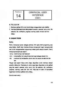
perform best as a model selection criterion for two-mode partitioning, in the sense that it indicated the true number of row and column clusters—which are known in a simulation study—most often. This convex hull procedure is incorporated in TwoMP in order to allow the user to choose a solution on the basis of the current best model selection criterion for two-mode partitioning. We will briefly describe the sequence of steps involved in the convex hull procedure here. First, a set of solutions with different numbers of row and/or column clusters are fitted to the data set in question. Next, for each of these solutions, the rank (P,Q) is mapped to a single complexity measure C by taking the sum P 1 Q. This implies that a single complexity value C may be associated with more than one VAF value. In order to explain the following steps, it is useful to consider a plot of VAF against C in which each solution corresponds to one point (see Figure 1A for a hypothetical example of such a plot). In a next step, only those solutions are retained that lie on the upper boundary of the convex hull of this plot (these solutions are indicated by a diamond and are connected by the solid line in Figure 1B). This subset of solutions is then ordered according to their complexity C, and the solution C b is looked for that shows the largest elbow. The latter implies that the ratio of the slope between C b21 and C b and the slope between C b and C b11 is the largest: in other words, the solution that itself implies a large increase in VAF, as compared with the previous solution, but after which the increase in VAF for the next solution is relatively small (in Figure 1, this clearly corresponds to the solution with C equal to 4). Finally, the particular solution of rank (P,Q) that corresponds to the elbow point with complexity C b is returned as the selected solution with the best trade-off between model complexity and data fit. TwoMP In this section, we will illustrate the functioning of TwoMP by making use of a small hypothetical data set. In

B 60

50

50

40

40

VAF

VAF

A 60

30

30

20

20

10

10

0

2

4

6

C

8

0

2

4

6

8

C

Figure 1. Graphical aid for understanding the convex hull procedure. VAF, percentage of variance accounted for.

510     Schepers and Hofmans Table 1 Hypothetical Situation by Behavior/Emotion Data Matrix

Situation Line at post office Group therapy Train Concert Work Visit parents Argument with spouse Therapist Home alone with pet dog Creativity therapy

Happy 3 2 1 3 6 2 1 3 5 6

Calm 0 1 2 1 7 2 2 2 5 4

Anxious 7 1 4 5 2 3 2 3 3 1

Obsessive Thoughts 7 3 6 5 1 3 3 4 1 1

Hyperventilating 6 2 7 6 1 2 1 2 3 3

Low SelfEsteem 6 5 6 8 1 7 7 6 2 3

Suicidal Thoughts 3 6 4 2 2 6 7 6 2 2

Anger 2 6 2 3 1 5 6 5 3 5

Incapability 8 8 8 5 2 7 7 6 3 2

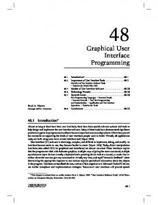
Regarding the data file, TwoMP accepts ASCII data files in which the columns are tab or space delimited, the rows are separated by line breaks, and decimal separators are denoted by a period. Only full data matrices, without Hypothetical Example missing values, are allowed. As a guiding example, we will make use of the (hypoProviding labels for both modes can be done by typthetical) data matrix shown in Table 1. These data represent, ing the labels in the corresponding “Row-set label” for a single person, the level at which a set of behaviors/­ and “Column-­set label” boxes. In our example, the row emotions (columns) is associated with a set of situations mode is defined as “Situations,” and the column mode as (rows).4 “Behaviors/­Emotions” (see Figure 2). If no labels are proIn the context of a personality diagnosis, such a data vided, TwoMP uses the default values “Rows” and “Colset may be collected in order to study how the profile of umns.” Specifying a location for the individual row and behaviors/emotions of a person varies over different situ- column labels is also optional; if the “Row Labels” option ations, which may then assist in determining an individu- is unspecified, TwoMP uses default labels for all rows (i.e., ally tailored treatment strategy. Although the size of our from “1” to the total number of rows in the data file, starting hypothetical data set is very modest (i.e., 10 3 9), this from the top row and labeling each next row in ascending example already shows that it is not easy to capture in order), and the same goes if the “Column Labels” option is an insightful way the information present in Table 1. In unspecified (i.e., starting from the leftmost column). Howparticular, just by looking at the values in Table 1, it is ever, if the user wishes to specify labels for the rows, the not easy to distinguish between the important information columns, or both, he or she must specify the location for (i.e., structural) and the unimportant information (e.g., the labels in question by using the appropriate “Browse” noise). One can imagine that this task becomes even more button. For example, in Figure 2 the names of the row and difficult for larger matrices. Two-mode partitioning of- column labels files are “c:\Situation_­BehaviorEmotion\ fers a solution by distinguishing groups of similar row RowLabels.txt” and “c:\Situation_­BehaviorEmotion\­ elements (i.e., situations) and groups of similar column ColumnLabels.txt,” respectively. Like the data file, labels elements (i.e., behaviors/emotions). files also should be in ASCII format. All labels should be separated by a line break. The label on the first line of the Program Handling labels file is associated with the first element of that mode. After starting MATLAB, TwoMP can be launched by For example, in a row label file, the label on the first line typing “TwoMP” after the command prompt (make sure is associated with the first row element (i.e., with the first that the current MATLAB directory is in the folder where row in the data matrix); in a column label file, the label on you have saved the TwoMP program files): the first line is associated with the first column element (i.e., with the leftmost column of the data matrix). Every >>TwoMP . next row/column is associated with the label in the next As a result, a graphical user interface (GUI) appears (see line of the row/column labels file. Figure  2). The GUI is subdivided into three compartIf a row/column label file is specified, the user should ments—that is, input, processing, and output—which will take care that every row/column is associated with exactly be discussed in the following paragraphs. one label: If the number of row labels in the row labels file Input. The input compartment allows the user to spec- does not coincide with the number of rows in the data file, ify the location of the data file, which is “c:\­Situation_ an error message is displayed at the command prompt, BehaviorEmotion\data.txt” in Figure 2. In addition, user- and likewise if the number of column labels in the column ­defined labels for the two modes—or the whole set of labels file does not coincide with the number of columns rows/columns—as well as row and column label files con- in the data file. TwoMP does not allow that only part of the taining labels for the individual rows and columns, may rows/columns should be labeled by providing a label file be specified. and the remaining part by default: Either a label file that practice, however, one will usually be interested in analyzing much larger data sets, because, in that case, the advantage of reducing both modes is most apparent.3

TwoMP MATLAB Graphical Interface     511

Figure 2. Screenshot of the graphical user interface of TwoMP.

contains a single label for every row/column is specified, or no label file should be specified at all, in which case TwoMP uses default labeling. Processing. The processing compartment allows the user to specify ranges for the number of desired row and column clusters, as well as the desired accuracy with which the clustering solutions are estimated. As in the traditional k-means clustering case, it is usually not known beforehand how many clusters one should expect in the data. A common procedure is, then, to estimate clustering solutions for a range of clusters. By default, TwoMP sets the minimal number of desired row and column clusters to 1 and the maximal number to 4. This implies that, for a given number of column clusters, all two-mode partitioning solutions are estimated, with the number of row clusters varying from 1 to 4. Similarly, for a given number of row clusters, all two-mode partitioning solutions are estimated, with the number of column clusters varying from 1 to 4. Consequently, by combining all possible values for the numbers of row and column clusters, in the default setting a total of 4 3 4 5 16 two-mode partitioning solutions are estimated. The user can change the range of desired clusters for both the rows and columns by specifying different values in the appropriate boxes. If only a single solution is desired—say, with three row clusters and four column clusters—both the

minimal and the maximal number of row clusters should be set equal to three. Similarly, both the minimal and maximal number of column clusters should then be set equal to four. To illustrate, this particular case is depicted in Figure 2. The “Number of Restarts” box allows the user to specify a desired accuracy of estimation. In general, the higher this number, the more accurate the estimated solution will be. Accuracy here refers to how close the VAF of an estimated solution is to the highest VAF of all possible solutions for a given number of row and column clusters. Even a robust optimization algorithm, such as the one implemented in TwoMP, may end up in a local optimum; that is, it does not necessarily return the solution with the highest VAF (Schepers et al., 2006). One may note that this is not specific to the two-mode partitioning problem but is also true for algorithms in the case of traditional k-means clustering (Hand & Krzanowski, 2005; Selim & Ismail, 1984; Steinley, 2003). In order to overcome this local optima problem, the optimization algorithm may be restarted using different starting values for the initial cluster assignments, which, in TwoMP, are drawn independently and identically from a discrete uniform distribution. Running time of TwoMP, however, increases with increasing numbers of restarts. Therefore, in practice, one should look for an “optimal” trade-off between desired accuracy and computation time. On the basis of the results reported in Schepers et al. (2006),

512     Schepers and Hofmans

Figure 3. Screenshot of part of the output file “model_3x4.mht.”

we believe that 50 restarts (which is also the default value in TwoMP) will usually lead to accurate results, while still being feasible in terms of running time. Output. The output compartment allows the user to specify where the output files (see the following section for more information on these output files) produced by TwoMP should be stored. This location can be either an existing folder or one that is to be created by TwoMP. The latter option can be achieved by clicking on the “Browse” button and following the subsequent instructions. In Figure 2, all output files produced by TwoMP will be stored in the folder “c:\Situation_BehaviorEmotion\Output.” Understanding Output Files TwoMP produces separate “.mht” output files5 for every estimated solution—that is, for every combina-

tion of a number of row and column clusters. Every such output file contains the results of the clustering and is named so that it is clear for which row 3 column clusters combination it contains the results. For example, the “model_3x4.mht” file contains the results for the model with three row clusters and four column clusters. In particular, the user may find here (1) the percentage of VAF by the model, (2) the grouping of the rows, (3) the grouping of the columns, and (4) the core matrix G. Figure 3 shows the VAF (i.e., 82.9146) and the grouping of the rows (i.e., “Situation”) as presented in such an output file (i.e., “model_3x4.mht”). In this file, the grouping of the columns (i.e., “Behavior/Emotion”) is displayed similarly to the grouping of the rows. It can be seen from Figure 3 that, for example, the first situation cluster contains the elements “group therapy,” “visit to parents,” “argument with spouse,” and “therapist.” One may note that each of these situations is associated with a numerical value, given between brackets. This value indicates the proportional contribution of each situation to the unexplained (or error) part of the data and sums to 1 over all situations. A similar case holds for “Behavior/Emotion.” Consequently, relatively high values indicate that the model does not fit the data for the row/ column in question as well as it does those for the other rows/­columns. One may take this into account when interpreting the clustering. For example, the model does not fit the data for “group therapy” as well as it does those for the other situations in the first situation cluster, since it has the largest proportional contribution to the error (i.e., 0.10582) of all four situations in this cluster. Every output file includes the results for the core matrix G as well. This matrix reports the strength of the relation between each row and column cluster. For the model with three row clusters and four column clusters, the core matrix is depicted in Figure 4. From this matrix, it can be seen that the first row cluster is associated with the first column cluster with a strength of 6.6250. As such, the core matrix G represents a summary of the observed data. Since this matrix contains considerably fewer rows and columns (i.e., 3 3 4) than does the observed data matrix (i.e., 10 3 9), it implies a reduction of the complexity of the original information. Apart from identifying the underlying groups of rows and columns, looking at the values in this core matrix may facilitate the interpretation of the structural information present in the observed data. When more than three solutions with different numbers of row and column clusters are estimated for the data,

Figure 4. Screenshot of the core matrix as included in “model_3x4.mht.”

TwoMP MATLAB Graphical Interface     513 Percentage of explained variance (VAF) for each model: nr. of Groups

Perc. of Explained Variance

1x1 1x2 1x3 1x4 2x1 2x2 2x3 2x4 3x1 3x2 3x3 3x4 4x1 4x2 4x3 4x4

0.00 14.41 16.40 17.18 7.79 44.15 59.36 61.44 8.56 45.91 70.35 82.91 8.83 47.39 72.20 84.80

Solutions on the convex hull and their fit (VAF) and 'elbow' value: 1x1 2x2 2x3 3x4 4x4

0.0000 44.1521 59.3629 82.9146 84.8048

0.0000 1.4513 1.2917 6.2299 0.0000

Best solution in terms of trade-off between complexity and fit: 3x4 Figure 5. Content of the “ModelSelection.doc” file .

TwoMP also produces an output file for model selection purposes. This file, “ModelSelection.doc,” reproduces the VAFs for each estimated solution and informs the user about which of these solutions is most promising in terms of a useful description of the data set in question. To identify the most promising solution, TwoMP relies on a convex hull procedure (Ceulemans & Van Mechelen, 2005; Schepers et al., 2008), as described in the Two-Mode Partitioning section. The “ModelSelection.doc” file contains three sections (see Figure 5): The first section includes a list of all estimated solutions (labeled by their respective number of row and column clusters) and their corresponding VAFs; the second section lists a subset of only those solutions that are considered most promising (i.e., those solutions that lie on the upper boundary of the convex hull of a plot of VAF against C ), along with their associated elbow values; the final section includes only that solution that is optimal in terms of the trade-off between model complexity and fit (i.e., the solution that, in the second section, shows the largest elbow). For our example, the solution with three Situation clusters and four Behavior/ Emotion clusters is identified as the most promising one. Summary TwoMP is a MATLAB GUI for two-mode partitioning analysis. It is freely available and easy to use and allows the user to perform a full two-mode partitioning analysis on a given data set by making use of an optimization algorithm (Gaul & Schader, 1996; Schepers et al., 2006),

supplemented by a validated model selection criterion (Schepers et al., 2008). Author Note The research reported here was supported by the Fund for Scientific Research–Flanders (Belgium), Project No. G.0146.04, awarded to Iven Van Mechelen, and by the Belgian Federal Science Policy (IAP P6-03). We are grateful for the comments and suggestions of two anonymous reviewers, which led to significant improvements to the final version of this article. Correspondence concerning this article should be addressed to J. Schepers, Faculty of Psychology and Neurosciences, Maastricht University, P.O. Box 616, 6210 MD Maastricht, The Netherlands (e-mail: [email protected]). References Baier, D., Gaul, W., & Schader, M. (1997). Two-mode overlapping clustering with applications to simultaneous benefit segmentation and market structuring. In R. Klar & O. Opitz (Eds.), Classification and knowledge organization (pp. 557-566). Berlin: Springer. Carroll, J. D., & Arabie, P. (1980). Multidimensional scaling. Annual Review of Psychology, 31, 607-649. Castillo, W., & Trejos, J. (2002). Two-mode partitioning: Review of methods and application of tabu search. In K. Jajuga, A. Sokolowski, & H.-H. Bock (Eds.), Classification, clustering, and related topics: Recent advances and applications (pp. 43-51). Heidelberg: Springer. Ceulemans, E., & Kiers, H. A. L. (2006). Selecting among three-mode principal component models of different types and complexities: A numerical convex hull based method. British Journal of Mathematical & Statistical Psychology, 59, 133-150. Ceulemans, E., & Van Mechelen, I. (2005). Hierarchical classes models for three-way three-mode binary data: Interrelations and model selection. Psychometrika, 70, 461-480. Gaul, W., & Schader, M. (1996). A new algorithm for two-mode clus-

514     Schepers and Hofmans tering. In H.-H. Bock & W. Polasek (Eds.), Classification and knowledge organization (pp. 15-23). Berlin: Springer. Hand, D. J., & Krzanowski, W. J. (2005). Optimising k-means clustering results with standard software packages. Computational Statistics & Data Analysis, 49, 969-973. Hartigan, J. A. (1975). Clustering algorithms. New York: Wiley. Kiers, H. A. L. (2004). Clustering all three modes of three-mode data: Computational possibilities and problems. In J. Antoch (Ed.), ­COMPSTAT: Proceedings in Computational Statistics (pp. 303-313). Heidelberg: Springer. MacQueen, J. (1967). Some methods for classification and analysis of multivariate observations. In L. M. Le Cam & J. Neyman (Eds.), Proceedings of the Fifth Berkeley Symposium on Mathematical Statistics and Probability (Vol. 1, pp. 281-297). Berkeley: University of California Press. Rocci, R., & Vichi, M. (2008). Two-mode multi-partitioning. Computational Statistics & Data Analysis, 52, 1984-2003. Schepers, J., Ceulemans, E., & Van Mechelen, I. (2008). Selecting among multi-mode partitioning models of different complexities: A comparison of four model selection criteria. Journal of Classification, 25, 67-85. Schepers, J., Van Mechelen, I., & Ceulemans, E. (2006). Threemode partitioning. Computational Statistics & Data Analysis, 51, 1623-1642. Selim, S. Z., & Ismail, M. A. (1984). K-means type algorithms: A generalized convergence theorem and characterization of local optimality. IEEE Transactions on Pattern Analysis & Machine Intelligence, 6, 81-87. Steinley, D. (2003). Local optima in K-means clustering: What you don’t know may hurt you. Psychological Methods, 8, 294-304. Timmerman, M. E., & Kiers, H. A. L. (2000). Three-mode principal components analysis: Choosing the numbers of components and sensitivity to local optima. British Journal of Mathematical & Statistical Psychology, 53, 1-16.

Van Mechelen, I., Bock, H.-H., & De Boeck, P. (2004). Two-mode clustering methods: A structured overview. Statistical Methods in Medical Research, 13, 363-394. Van Mechelen, I., & Schepers, J. (2007). A unifying model involving a categorical and/or dimensional reduction for multimode data. Computational Statistics & Data Analysis, 52, 537-549. van Rosmalen, J., Groenen, P. J., Trejos, J., & Castillo, W. (2005). Global optimization strategies for two-mode clustering (Rep. EI ­2005-33). Rotterdam: Erasmus Universiteit Rotterdam, Econometric Institute. Notes 1. A partition matrix is a binary matrix of which each row sums to one and in which no zero columns are observed. 2. As an aside, one may note that the algorithms proposed in Kiers (2004) and Schepers et al. (2006) even allow for an additional third mode in the data to be reduced. 3. It is difficult to specify an exact upper bound on the maximum size of data sets that TwoMP can handle properly. This is because for very large data sets, TwoMP may, due to its combinatorial nature, require extremely long running times. However, we believe that in applications in the social sciences, data matrices usually do not exceed, say, 500 rows 3 100 columns. Running times associated with applications of this size are still within an “acceptable” range. 4. TwoMP is by no means restricted to data sets of this particular type (i.e., situation by behavior/emotion). In general, the rows and columns of the data matrix may represent any set of “research units.” For example, in many applications in psychology, the rows represent the set of participants in a study. 5. These files can be opened using standard software such as Microsoft Word or Internet Explorer. (Manuscript received July 9, 2008; revision accepted for publication December 15, 2008.)