Building a Simulation Environment for Optimising Control ... - CiteSeerX

th

Proceedings of the 9 Chinese Automation & Computing Society Conference in the UK, Luton, England, 20 September 2003

Building a Simulation Environment for Optimising Control Parameters of an Autonomous Robotic Fish Jindong Liu and Huosheng Hu Department of Computer Science, University of Essex Wivenhoe Park, Colchester CO4 3SQ Email: [email protected], [email protected] Abstract-- This paper firstly presents a short review on the current research of robotic fish. The construction of a simulation environment for robotic fish is then presented. The experiment results show that the simulator is a convenient way to develop and test the motion control algorithm for a robotic fish. Furthermore, a parameter optimising method for fish’s travelling wave approximation is proposed. A special error function is selected depending on the hydrodynamics theory of fish.

Table 1 lists the most of researches on robotic fish in the world. Table 1: The robotic fish research in the world Nation

MIT

U.S.

I. INTRODUCTION

I

n nature, fish has astonishing swimming ability after thousands years evolution. It is well known that the tuna swims with high speed and high efficiency, the pike accelerates in a flash and the eel could swims skillfully into narrow holes. Such astonishing swimming ability inspires the researchers to improve the performance of aquatic man-made systems. An example application is robotic fish. Instead of the conventional rotary propeller used in ship or underwater vehicles, the undulation movement like fish provides the main energy of the robotic fish. The observation on the real fish shows that this kind of propulsion is more noiseless, effective, and manoeuvrable than the propeller-based propulsion. So, the robotic fish could be used in many marine and military fields such as exploring the fish behaviours, detecting the leakage of oil pipeline, robotics education, mine countermeasures, etc. In 1994, the first robot fish named robotuna was developed by MIT [2]. In 1998, the Draper Lab realized Vorticity Control Unmanned Undersea Vehicle (VCUUV) [3] on the base of robotuna. VCUUV could avoid obstacle and realize the up-down motion. It is the most widely known robotic fish developed up to now. After that, many researchers put forward several kinds of robot fish. The Northwestern University applied Shape Memory Alloy (SMA) on the robotic lamprey [6] which make aim to realize mine countermeasures. In Japan, Nagoya University developed a kind of micro robotic fish using ICPF Actuator [7] and Tokai University realized a robotic Blackbass [5] to research the propulsion of pectoral fins. National Maritime Research Institute of Japan developed many kinds of robotic fish prototypes from PF300 to PPF09 [8] to exploit the up-down method and effective swimming. In China, the Beihang University (BUAA) developed three kinds of robotic fish [9] and the Institute of Automation Chinese Academy of Sciences (CASIA) [10] also made some progress on four-joint robotic fish.

Researcher

Northeastern University California Technology Institute University of New Mexico

U.K

Japan

Project Robotuna(1994) [2], VCUUV(1998) [3] robotic lamperry [6] Sensors and Control of Robot fish [4] The application of IEM and artificial muscle on the robotic fish [13]

Heriot-Watt University National Maritime Research Institute Tokai University

PF-300, PF-600, PPF-09, PF-700, UPF-2001 [8]

Nagoya University

Microroobt using ICPF Actuator [7]

BUAA

mini-robofish and SPC [9]

CASIA

Robofish [10]

Professor Dan Mssie

Robotic fish named Dongle [14]

FLAPS project [1]

Robot Blackbass [5]

China

Other

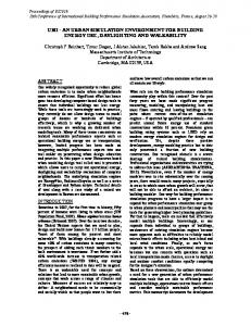
Most of previous research focused on the hydrodynamics mechanism of fishlike swimming, the special skin material and mechanical structure of robotic fish models. Although, for future application, autonomous motion control is definitely necessary for robotic fish, there is almost no person to do research on it. The aim of the project described in this paper is to design and build an autonomous navigation robotic fish. The robotic fish would have two main features: to swim like real fish and to realize autonomous motion control. Two of optimal elements are intelligent motion control algorithm and fish-like motion parameters. Here, a simulation environment is built up in Part II to explore an efficient autonomous navigation algorithm based on the four-joint robotic fish of CASIA (Figure 1). Furthermore, a parameter optimisation method for fish’s travelling wave approximating is proposed in Part III. A special error

317

function is selected depending on the hydrodynamics theory of fish. Two experiments are given in Part IV. Finally, section V summarizes the research progress and potential future development. II. SIMULATION ENVIRONMENT To study the kinematic and hydrodynamic theory, a virtual swimming pool and robotic fish have been built based on a robotic fish in our lab. The main targets of the simulation work are: • To simulate the hydrodynamic model of a robotic fish, to understand the relationship between the movement of the fish tail and the forces acting on fish. • To develop fish-like motion control algorithms for the robotic fish, to realize or mimic the real fish behaviours such as decelerating/accelerating swim, constant swim, turning and hover. • In large noise situation (the wave effect), to test the algorithms of artificial intelligence in robotic fish such as to avoid obstacle, to pursue a moving target, to swim in an appointed trace, etc.

responsibility is to transfer the command and initial object data from users to Data Layer. It also could display the real-time update of objects on the screen. Figure 2 shows an example of user interface. The whole simulation environment is built by the “Object Oriented” programming method, i.e. C++ is selected as the program language. Sonar(L,R)

Joint1...4

Obstacle 1...10

Robotic Fish Ambient, Task&Noise data; Control command

Ambient

Fish & Joint Status

Object layer

Task Ambient Update data from user

Update from user

Task Update data from user

Data Exchange Centre Data of fish, ambient & task User Set Interface

Set Fish Set Ambient

Set Task

Command

Noise data

Data layer Data Update

User Control Interface

Set Noise

Noise

Control Command

Data Update

Data Display (Monitor)

User Interface layer User

Figure 3.The simulation environment

Figure 1 The Robotic Fish

Figure 2. The simulation Environment

A. Components of Simulation Environment Figure 3 shows the main frame of the simulator that consists of: Object Layer, Data Layer and User Interface Layer. The Object layer consists of all virtual objects in the simulator such as robotic fish, sonar, fish joints, ambient, obstacles, task and noise. The virtual robotic fish includes sonars and joints. The ambient describes the virtual swimming pool in which the robotic fish swims. It includes several obstacles, which are simplified as round shape. The task records the appointed trace that the robotic fish is expected to follow. The noise simulates the disturbance of water when the robotic fish swims. The Data Layer is a data exchange centre. All virtual environment data is stored and exchanged by it. It is also a connector between User Interface Layer and Object layer. The User Interface Layer is an interactive layer between users and the simulation environment. Its

The virtual robotic fish has three main components: head, 4 joints and 2 sensors. Each fish joint is viewed as a quadrilateral, which is defined by four vertexes. It could rotate at the base point by a relative angle related to the anterior joint. Where, the base point is the centre of the conjunct line of two adjacent joints. In the real world, the base-point is the position to fix the joint motor. Figure 4 shows a fish joint transformation when a robotic fish swims. The joint will first rotate θ following the fish head and then rotate ϕ at its axle. Figure 5 gives a posture of robotic fish by appointing the heading, the relative angle between Joint_I.vs.Head, Joint_II.vs.Joint_I, Joint_III.vs.Joint_II, Joint_IV.vs.Joint_III. An angle set Φ denotes the above four relative angles. When the Φ changes as some wave function, the virtual robotic fish will swim like real fish. See the Part III for details. y

Χ0 Χ1

ϕ

θ

Y0 Y1

0

x

Χ2

Figure 4 Joint Transformation

Figure 5. A virtual robotic fish

Two sonar sensors are fixed on the “eyes” position of the virtual fish. The virtual sonar sensor (Figure 6-B) is built up on the base of real sonar sensors (Figure 6-A[15]). The transducer and the receiver are viewed as a same point. A bunch of rays is created at the front of the T/R

318

point to simulate the ultrasonic wave. When the robotic fish try to detect obstacle by sonar, just to compute the crossing point of each ray with the obstacle in ambient.

Lighthill’s “Large-amplitude elongated-body theory”[12] is selected as the basic theory of hydrodynamic model. The detail of (K&D model) is shown in Figure 8. Detect Obstacle by sonar

Fish Status i

Sonar Data

Task

θ

Pre-procession on sonar data

Obstacle Data

Task Compare Model ∆ Task

(A)

T/R Virtual Sonar Model (B)

Fish Behaviours Library

Figure 6.The sonar model in our robotic fish

There are three types of task: free swimming, static trace and dynamic trace. In this paper, the experiment is limited in the free-swimming task. The robotic fish wanders in a swimming pool without a goal. In every data update cycle of robotic fish, a random command is sent out. The aim of such task is to test the ability of avoiding obstacle and detecting pool border.

Note: ∆ Task is the difference between current position and expected task

Behaviour Decision Explain Model Expected Aˆti +1, Aˆ ri +1

Kinematic and Hydrodynamic Model

Fish&Joint Status i+1

B. Computation in Virtual Robotic Fish

In simulation, an “Update Cycle” is predefined to control the update of the status of robotic fish and fish joints in real time, where, the status means kinemics information such as position and velocity. Figure 7 shows the main components in one of update cycles. There are six processing models and one fish behaviours library. The detailed process can be described as follows: First, the robotic fish gets itself current status that includes position, fish heading, linear velocity, angular velocity, linear acceleration, angular acceleration and the time of last updating. The “Task Compare” model is called to compare the current fish position with the expected trace, i.e. task, and outputs the ∆ Task for “Make Decision” model. Then the “Detect Obstacle” model and “Preprocession” model are called to get the obstacle direction and distance. Third, in “Make Decision Model” the robotic fish makes decision depending on the obstacle information and the result from task compare model. The decision is limited in the scope of “Fish Behaviours Library” which stores all possible fish-like behaviours. Fourth, the robotic fish transforms the decision into the expected linear acceleration and angular acceleration for the next time. Finally, in “Kinematic and Hydrodynamic Model (K&D model)”, the robotic fish computes the hydrodynamic parameter to get the “real” linear acceleration and angular acceleration from the expected. Then the status of robotic fish and joint for next time are obtained from kinematics model. The reason of why the expected Aˆti +1, Aˆ ri +1 may be different from the real Ati +1 , Ari +1

Make Decision Model

is caused by the mechanical limitation of real robotic fish and its special hydrodynamic feature.

Figure 7.Update Cycle for fish and joints

Fish Status i+1

Fish Status i

Real Ati +1 , Ari +1 Expected Aˆti +1, Aˆ ri +1

ϖ i +1

Joints Status i

Joints Status i+1

Note: Ati +1 , Ari +1 are the linear speed and rotational speed of robotic fish respectively. ϖ i +1 is the phaseangle between Joint Statutes i and Joint Status i+1. The ˆ i +1, Aˆ i +1 are the result of Decision Model. expected A t r

Figure 8 The Kinematic& Hydrodynamics Model of our robotic fish

III. PARAMETER OPTIMISATION The motion of fish tail could be described by a travelling wave (1) which was originally suggested by Lighthill [11]. The original point of (1) is set at the conjunction point between fish head and tail. The parameter of travelling wave changes depending on the kind of fish and the fish kinetics status in water. So, the swimming of fish could be viewed as making the fish body approximate the travelling wave. For real fish, it has tens of vertebras that could be viewed as tens of mini joints to approximate the wave. So

319

the approximate result is very smooth. But for our robotic fish, it only has four joints, which is impossible to generate smooth wave. How to use limited joints to approximate the travelling wave in minimal error is the topic discussed in this paragraph.

y body ( x, t ) = ( c1 x + c 2 x 2 ) sin( kx + ωt ) where

y body

transverse displacement of tail unit;

displacement along main axis;

k=

2π

λ

“End_Point”. The function of line L is defined as y = g (x ) . So we get following two terms: Cross _ x

Positive _ Re g =

[g ( x ) − f ( x)]dx

(3)

Base _ x

(1)

End _ x

Negative _ Re g =

x

[g ( x ) − f ( x )]dx

(4)

Cross _ x

wave number; λ

wave length; c1 linear wave amplitude envelope; c2 quadratic wave amplitude envelope; ω = 2πf wave frequency. t time. In [16], a discrete travelling wave is considered and time t is separated from (1) in order to simplify the control method on joint motors of robotic fish. The rewritten equation is (2) in which the original travelling wave is decomposed into two parts: the time-independent wave sequence ybody ( x, i )(i = 0,1,..., M − 1) in an oscillation cycle and the time-dependent oscillation frequency f . y body ( x, i ) = ( c1 x + c 2 x 2 ) sin( kx −

2π i) M

i ∈ [0, M − 1]

Figure 10 an example of travelling wave approximation

(2) where i is serial number in an oscillation cycle. M is the resolution of discrete travelling wave. Figure 9 is an example for one oscillation cycle at M = 18 . Figure 10 shows an approximating result by four joints. The “I…IV” is the joint number. It is clear that the end point of each joint is the key element for travelling wave approximating. In [16], the method to find an end point assumed that each point falls onto the travelling curve. But we found that its error is large. Here, a special error function is proposed, based on the hydrodynamic theory of fish and a simple computation method is applied to get end points. Figure 9 An oscillation cycle at M = 18 .

Before discussion, it is necessary to define some special terms. See Figure 11. When a length-fix line L

which starts from “Base_Point” trys to approximate a curve defined as y = f (x ) , assume the first crossing point from “Base_Point” between L and y = f (x ) as “Cross_Point”. Another end of L is defined as

y Negative Reg End_Point Base_Point y=f(x) L Cross_Point Positive reg x Base_x Cross_x End_x Figure 11 Term definitions

There are two main methods to explain how the thrust force is generated for a fish: an added-mass method and a lift-based (vorticity) method[1]. The Carangiform mode that our robotic fish belongs to is associated with the added-mass method. As the propulsive wave passes backward along the fish, the momentum of the water passing backward is changed by the movement of the fish tail, which causes a reaction force FR from water to fish. FR is analysed into a lateral FL and a thrust FT component which contributes to forward propulsion for fish. The mass of the water passing backward is called added-mass. Its magnitude is partly depending on the wave of the fish tail. When using a length-fix joint to approximate a wave of fish tail, the ideal situation is to make the added-mass pushed away by joint equal to one by wave. In other words, we have Positiv _ Re g + Negative _ Re g = 0 . So the following error function is selected for travelling wave approximation instead of common quadratic error function.

320

an End_Point position (End _ xi, j , End _ yi, j ) Rc0 is easy to get

End _ x

[g ( x ) − f ( x )]dx

e( x ) = Positive _ Re g + Negative _ Re g =

and the parameter in (6) is determined for Rc0 . Finally, a ei, j ( x ) Rc0 could be obtained.

Base _ x

(5) When applying four joints to approximate the travelling curve, the task is to find a series of “End_Point” to minimize the

If

Rc = Rc 0 , Rc1, Rc 2 ,..., Rcn

approximate minimal

ei , j min

StepR = 1

n

, an

could be compute as:

ei , j min = Min ( ei , j ( x ) Rck ) . k =0...n

End _ xi , j

ei , j ( x ) =

is set by step

[ gi, j ( x ) − fi ( x )]dx (i = 0,2...M − 1, j = 1,2,3,4)

where f i ( x ) = y body ( x, i ) End _ yi, j − Base _ yi, j End _ xi, j − Base _ xi, j

an

is set as the

could be obtained easily. The will be used for joint motor control in a robotic fish directly.

bi, j = Base _ yi , j − ki , j Base _ xi , j

example)

Jo int_ Angle[ M ][4]

The constraint function is: Base _ xi , j = Base _ yi , j = 0 j = 1 Base _ xi , j = End _ xi , j −1 j = 2 ,3,4 2

IV. EXPERIMENT A. Simulation Experiment

( End _ xi , j − Base _ xi , j ) + ( End _ yi , j − Base _ yi, j ) = l 2j

2

where l j is the length of joint j . It is difficult to get analytic solutions from (5). So we seek for the numerical solution by MatLab. A crossing ratio is defined as Rc =

(End _ xi, j , End _ yi, j ) Rck

final result for joint j & serial number i . By using same method, a 2D array End _ Po int[M ][4] will be achieved and a corresponding Jo int_ Angle[ M ][4] which stores the joint relative angle θi, j (see Figure 10 for

Base _ xi , j

gi, j ( x ) = ki, j x + bi, j , ki , j =

The corresponding

(6)

Cross _ xi, j Base _ xi , j

, Rc ∈ [0,1] ,

Figure 12 is a video sequence for the simulation experiment being built. The robotic fish is trying to finish a “Free Swimming” task to test a simple motion control algorithm. When the virtual fish swims, its joint data is recorded for future analysis. B. Parameter Optimisation Result

an equations sets is defined as:

( )

( x − Base _ xi , j )2 + ( y − Base _ yi, j )2 = Rcl j 2π y = ( c1x + c2 x 2 ) sin( kx − i) M i = 1,2...M − 1, j = 1,2,3,4

2

(7)

Figure 13 is an example that applies four joints to approximate some travelling wave when M = 18 and Step R = 1 . The signal “ ∆ ”s show the End_Point of each 10

For a given Rc = Rc0 , the equations sets 7 could be solved by iterative method, i.e. a Cross_Point position for Rc 0 . Then

joint. The 8-shape curves are the trace of End_Point in one cycle. Figure 14 is two curves of error sum .vs. serial num. i.e.: 4

Sum error (i ) =

ei, j min , i = 0,2....17 j =1

(a)

(e)

(b)

(c)

(f) (g) Figure 12. An Experiment of Free Swimming

321

(d)

(h)

(8)

REFERENCES

Figure 13 an example of travelling wave approximation

Figure 14 Error Sum Curve Sumerror (18) = Sumerror (0) ,

the error curve A is the result of the method in[16] and the error curve B is the result of the new method in this paper. V. CONCLUSION AND FUTURE WORK A simulation environment for optimising control parameters of a robotic fish is described in this paper. The experimental results have shown that the simulation environment is a convenient method to design and optimise control parameters for motion control of robotic fish. The new method to compute End_Point has less error than the traditional method. In future, we would optimise the parameters: C1 , C 2 , k for the robotic fish to achieve high efficiency of thrust. Furthermore, the motion control method for other kinds of task will also be investigated, such as pass through a narrow gap and push a ball into a goal. VI. ACKNOWLEDGEMENT Our thanks go to Dr. Wang Shuo and Dr. Yu Junzhi for their robotic fish platform.

[1] M. Sfakiotakis, etc. “Review of Fish Swimming Modes for Aquatic Locomotion. IEEE Journal of Oceananic Engineering”. 1999,24(2): 237-252 [2] K. Streitlien, G. S. Triantafyllou, and M. S. Triantafyllou, “Efficient foil propulsion through vortex control,” AIAA J., vol. 34, pp. 2315–2319, 1996. [3] J.M.Anderson, “Vorticity control for efficient propulsion,” Ph.D. dissertation, Massachusetts Inst. Technol./Woods Hole Oceanographic Inst. Joint Program, Woods Hole, MA, 1996. [4] K.A. Morgansen, Vincent Duindam, Richard J. Mason. “Nonlinear Control Methods for Planar Carangiform Robot Fish Locomotion”. Proceeding of the 2001 IEEE International Conference on Robotics and Automation. pp 427-434. [5] N. Kato. “Control performance in the horizontal plane of a fish robot with mechanical pectoral fins”. IEEE Journal of Oceanic Engineering 25 1 2000 IEEE p 121-129 0364-9059 [6] http://www.dac.neu.edu/msc/burp.html [7] S. Guo, T. Fukuda, Norihiko KATO, Keisuke OGURO. “Development of Underwater Microrobot Using ICPF Actuator”. Proceedings of the 1998 IEEE International Conference on Robotics & Automation. pp1829-1834. [8] http://www.nmri.go.jp/eng/khirata/fish [9] J. Liang, etc. “Researchful Development of Underwater Robofish II- Development of a Small Experimental Robofish”. Robot .2002, 24(3) [10] J.Z. Yu, E.K. Chen, S. Wang, M. TAN, “Research Evolution and Analysis of Biomimetic Robot Fish”. Control Theory and Application. Accepted in Chinese.2002 [11] M. J. Lighthill, “Note on the swimming of slender fish,” J. Fluid Mech., vol. 9, pp. 305–317, 1960. [12] M. J. Lighthill, “Large-amplitude elongated-body theory of fish locomotion,” in Proc. R. Soc. Lond. B, 1971, vol. 179, pp. 125–138. [13] M. Mojarrad; M. Shahinpoor. “Noiseless propulsion for swimming robotic structures using polyelectrolyte ion-exchange membrane”. The International Society for Optical Engineering v 2716 Feb 26-27 96 1996 Sponsored by: SPIE - Int Soc for Opt Engineering, Bellingham, WA USA Society of Photo-Optical Instrumentation Engineers p 183-192 [14] http://www.seattlerobotics.org/encoder/200211/auto nomous_robotic_fish.html [15] B. Ayrulu and B. Barshan. “Reliability measure assignment to sonar forro bust target differentiation”. Pattern Recognition 35 (2002) 1403–1419. [16] J.Z. Yu, etc. A simplified Propulsive Model of Biomimetic Robot Fish and Its Realization. Submitted. [17] C.C. Lindsey, “Form, function and locomotory habits in fish”. Fish Physiology Vol. VII Locomotion. New York: Academic. 1978. pp.1-100.

322