Building Efficient Model Checkers using Hierarchical Set ... - Lip6

Fundamenta Informaticae Petri Nets (2008) 1–25

1

IOS Press

Building Efficient Model Checkers using Hierarchical Set Decision Diagrams and Automatic Saturation Alexandre Hamez Université P. & M. Curie LIP6 - CNRS UMR 7606 4 Place Jussieu, 75252 Paris cedex 05, France EPITA Research and Development Laboratory F-94276 Le Kremlin-Bicêtre cedex, France

Yann Thierry-Mieg Université P. & M. Curie LIP6 - CNRS UMR 7606 4 Place Jussieu, 75252 Paris cedex 05, France

Fabrice Kordon Université P. & M. Curie LIP6 - CNRS UMR 7606 4 Place Jussieu, 75252 Paris cedex 05, France

Abstract. Shared decision diagram representations of a state-space provide efficient solutions for model-checking of large systems. However, decision diagram manipulation is tricky, as the construction procedure is liable to produce intractable intermediate structures (a.k.a peak effect). The definition of the so-called saturation method has empirically been shown to mostly avoid this peak effect, and allows verification of much larger systems. However, applying this algorithm currently requires deep knowledge of the decision diagram data structures. Hierarchical Set Decision Diagrams (SDD) are decision diagrams in which arcs of the structure are labeled with sets, themselves stored as SDD. This data structure offers an elegant and very efficient way of encoding structured specifications using decision diagram technology. It also offers, through the concept of inductive homomorphisms, flexibility to a user defining a symbolic transition relation. We show in this paper how, with very limited user input, the SDD library is able to optimize evaluation of a transition relation to produce a saturation effect at runtime. We build as an example an SDD model-checker for a compositional formalism: Instantiable Petri Nets (IPN). IPN define a type as an abstract contract. Labeled P/T nets are used as an elementary type. A composite type is defined to hierarchically contain instances (of elementary or composite type). To compose behaviors, IPN use classic label synchronization semantics from process calculi. With a particular recursive folding SDD are able to offer solutions for symmetric systems in logarithmic complexity with respect to other DD. Even in less regular cases, the use of hierarchy in the specification is shown to be well supported by SDD. Experimentations and performances are reported on some well known examples.

Keywords Hierarchical Decision Diagrams, Model Checking, Saturation

2

A. Hamez, Y. Thierry-Mieg, F. Kordon / Efficient Model Checkers using Hierarchical Set Decision Diagrams

1. Introduction Parallel systems are notably difficult to verify due to their complexity. Non-determinism of the interleaving of elementary actions in particular is a source of errors difficult to detect through testing. Modelchecking of finite systems or exhaustive exploration of the state-space is very simple in its principle, entirely automatic, and provides useful counter-examples when the desired property is not verified. However model-checking suffers from the combinatorial state-space explosion problem, that severely limits the size of systems that can be checked automatically. One solution which has shown its strength to tackle very large state spaces is the use of shared decision diagrams like BDD [4, 5]. But decision diagram technology also suffers from two main drawbacks. First, the order of variables has a huge impact on performance and defining an appropriate order is non-trivial [3]. Second, the way the transition relation is defined and applied may have a huge impact on tool performance [19, 10]. Such aspects are difficult to tackle for non specialists of decision diagram technology. The objective of this paper is to present novel optimization techniques for hierarchical decision diagrams called Set Decision Diagrams (SDD), suitable to master the complexity of very large systems. Although SDD are a general all-purpose compact data-structure, a design goal has been to provide easy to use off the shelf constructs (such as a fixpoint) to develop a model-checker using SDD. These constructs allow the library to control operation application, and harness the power of state of the art saturation algorithms [10] with limited user expertise in DD. These high level constructs allow a user to concentrate on specifying the transition relation of the system using homomorphisms. The rewriting rules introduced in this paper allow to obtain an equivalent representation (with the same overall effect), but that optimizes its evaluation. No specific hypothesis is made on the input language, although we focus here on a system described as a composition of labeled transition systems. This simple formalism captures most transition-based representations (such as automata [1], communicating processes like in Promela [16] or Harel state charts [15]). To illustrate the use of our approach, we introduce IPN, a hierarchical Petri net representation as a basis for illustration and experimentation. Our hierarchical Set Decision Diagrams (section 2) offer the following capabilities: • Exploitation of specification’s structure to introduce hierarchy in the state space, it enables more possibilities for exploiting pattern similarities in the system, • Automatic activation of saturation; the algorithms described in this paper allow the library to enact saturation with minimal user input, • A recursive folding technique that is suitable for very symmetric systems. The paper is structured as follows. Section 2 presents SDD and section 3 defines a compositional Petri net formalism: Instantiable Petri Nets (IPN), that provide built-in functions for modularity and assembling. Section 4 then explains how to build a model checker for IPN on top of SDD. Sections 5 and 6 show how we can provide transparent optimizations, thus extending the saturation mechanisms introduced in [10]. Section 7 then presents a performance evaluation of our openly distributed implementation: libddd [18]. Finally, section 8 presents a way to take advantage of hierarchy in decision diagrams for very regular systems, as well as the associated performance results we get.


3

2. Hierarchical Set Decision Diagram (SDD) This section recalls the salient points of Hierarchical Set Decision Diagrams (SDD), a data structure based on the principles of decision diagram technology (node uniqueness thanks to a canonical representation, dynamic programming, ordering issues, etc.). They feature two main original aspects: the support of hierarchy in the representation (section 2.1) and the definition of user operations through a mechanism called inductive homomorphisms (section 2.2) which gives freedom and flexibility to the user.

2.1. Structure of SDD Hierarchical Set Decision Diagrams (SDD) defined in [13], are shared decision diagrams in which arcs are labeled by a set of values, instead of a single value. This set may itself be represented by an SDD, thus when labels are SDD, we think of them as hierarchical decision diagrams. Definition 2.1 is taken practically verbatim from [14] where it was adapted for more clarity from [13]. SDD are data structures for representing sets of sequences of assignments of the form ω1 ∈ s1 ; ω2 ∈ s2 ; · · · ; ωn ∈ sn where ωi are variables and si are sets of values. We assume no variable ordering, and the same variable can occur several times in an assignment sequence. We define the terminal 1 to represent the empty assignment sequence, that terminates any valid sequence. The terminal 0 represents the empty set of assignment sequences. In the following, Var denotes a set of variables, and for any ω in Var, Dom(ω) represents the domain of ω which may be infinite. Definition 2.1. (Set Decision Diagram) δ ∈ S, the set of SDD, is inductively defined by: • δ ∈ {0, 1} or • δ = hω, π, αi with: – ω ∈ Var. – π = s0 ∪ · · · ∪ sn is a finite partition of Dom(ω), i.e. ∀i , j, si ∩ s j = ∅, si , ∅, n finite. – α : π → S, such that ∀i , j, α(si ) , α(s j ). By convention, when it exists, the element of the partition π that maps to the SDD 0 is not represented. s We denote by ω → − δ′ , the SDD δ = hω, π, αi with π = s and α(s) = δ′ (and α(Dom(ω) \ s) = 0). Despite its simplicity, this definition supports rich and complex data: • SDD support domains of infinite size (e.g. Dom(ω) = R), provided that the number of elements in the partition remains finite (e.g. ]0..3], ]3.. + ∞]). This feature could be used to model clocks for instance (as in [21]). It also places the expressive power of SDD above most variants of DD. • SDD or other variants of decision diagrams can be used as the domain of variables, introducing hierarchy in the data structure.

4


• SDD can handle paths of variable lengths, if care is taken when choosing the state encoding to avoid creating so-called incompatible sequences (see [13]). This feature is useful when representing dynamic structures such as queues, lists or variable size arrays. The definition ensures that any set of assignment sequences has a unique (canonical) SDD representation. The finite size of the partition π ensures we can store α as a finite set of pairs hsi , δi i, and let π be implicitly defined by α. SDD are canonized by construction through the union operator. The canonicity of SDD is due to the two properties (1) π is a partition and (2) no two arcs from a node may lead to the same SDD. Therefore any value x ∈ Dom(ω) is represented on at most one arc, and any time we are about to construct s

s′

s∪s′

ω→ − δ + ω −→ δ, we will construct an arc ω −−−→ δ instead (fusing arcs). The opposite effect (splitting arcs) is obtained when building an SDD such that two arcs hs, δi and ′ hs , δ′ i have non empty intersection s ∩ s′ , ∅. We then produce three arcs, hs \ s′ , δi, hs′ \ s, δ′ i and hs ∩ s′ , δ ∪ δ′ i. To handle paths of variable lengths, SDD are required to represent a set of compatible assignment sequences. An operation over SDD is said partially defined if it may produce incompatible sequences in the result. Definition 2.2. (Compatible SDD sequences) s0 sn An SDD sequence is an SDD of the form ω0 −→ · · · ωn −→ 1. Let σ1 , σ2 be two sequences, σ1 ≈ σ2 iff.: • σ1 = 1 ∧ σ2 = 1    ω = ω′   ′  s s  • σ1 = ω → − δ ∧ σ2 = ω′ −→ δ′ such that  ∧s ≈ s′      ∧s ∩ s′ , ∅ =⇒ δ ≈ δ′ Compatibility is a symmetric property. The s ≈ s′ condition is defined as SDD compatibility if s, s′ ∈ S. Other possible referenced types should define their own notion of compatibility. While this notion of compatible sequences may seem restrictive, it is more permissive than usual for DD, where the norm is to use a fixed set of variables, in a fixed order along all paths. In practice, we use this compatible sequence definition to handle dynamic structures such as queues. To encode a queue, we repeat the same variable ω. The last occurrence of ω along any path is then artificially labeled ♯

s1

♯

with a special marker, noted ♯. Hence, ω → − 1 represents an empty queue, and ω −→ ω → − 1 represents a queue with one element (chosen from s1 ). These two SDD are compatible, and can be stored inside a single SDD. Furthermore, using homomorphisms we can define appropriate operations to manipulate such dynamic structures (see [12]).

2.2. Operations and Homomorphisms Usually in symbolic methods (e.g. BDD), the next state function of a system is encoded using one or more decision diagrams, with two variables per variable of the state signature. These variables are usually interlaced in the transition relation representation. A dedicated synchronized product operation then allows to compute the successor image for a set of states.


5

In contrast to BDD, SDD operations are encoded as homomorphisms S 7→ S. SDD support standard set theoretic operations (∪, ∩, \ respectively noted +, ∗, −). They also offer a concatenation operation δ1 · δ2 which replaces 1 terminal of δ1 by δ2 . This corresponds to a Cartesian product. In addition, basic and inductive homomorphisms are introduced as a powerful and flexible mechanism to define application specific operations. A detailed description of homomorphisms including many examples can be found in [12]. A basic homomorphism is a mapping Φ : S 7→ S satisfying Φ(0) = 0 and ∀δ, δ′ ∈ S, Φ(δ + δ′ ) = Φ(δ) + ′ Φ(δ ). The sum + and the composition ◦ of two homomorphisms are homomorphisms. For instance, the homomorphism δ · Id, where δ ∈ S and Id designates the identity homomorphism, permits to left concatenate sequences. Some basic homomorphisms are hard-coded. For instance, the homomorphism δ ∗ Id where d ∈ S, ∗ stands for the intersection and Id for the identity, allows to select the sequences belonging to d : it is an homomorphism that can be applied to any d′ yielding d ∗ Id(d′ ) = d ∩ d′ . The homomorphisms d · Id and Id · d permit to left or right concatenate sequences. We widely use the left s concatenation of a single assignment (ω ∈ s), noted ω → − Id. Furthermore, application-specific mappings can be defined by inductive homomorphisms over S. An inductive homomorphism φ is defined by its evaluation on the 1 terminal φ(1) ∈ S, and its evaluation φ(ω, s) for any ω ∈ Var and any s ⊆ Dom(ω). The expression φ(ω, s) is itself a (possibly inductive) homomorphism, that will be applied on the successor node α(s). The result of φ(hω, π, αi) is then defined P P as s∈π φ(ω, s)(α(s)), where represents a union. As an example, the local construction L allows to “carry” a homomorphism h to a certain variable v, and apply h to the current state of v. Thus, it implements an operation local to the variable v. This homomorphism will be used in section 4. It is defined by:  s    − L(v, h) if ω , v  ω→ L(v, h)(ω, s) =  h(s)    ω −−−→ Id else L(v, h)(1)

= 0

The reader will find several examples of homomorphisms throughout this paper. Section 6 shows simple homomorphisms that select and increment assignment sequences, while Section 4 shows more complex homomorphisms that describe the transition relation of a Petri net. The transitive closure ⋆ unary operator allows to perform a least fixpoint computation. For any homomorphism h and any node δ ∈ S, h⋆ (δ) is evaluated by repeating δ ← h(δ) until a fixpoint is reached. In other words, h⋆ (δ) = hn (δ) where n is the smallest integer such that hn (δ) = hn+1 (δ). This operator is often applied to (Id + h) instead of just h, allowing to accumulate newly computed assignment sequences in the result. An important contribution of [14] is the definition of a set of rewriting rules for homomorphisms, allowing to automatically make use of the decision diagram saturation algorithms originally due to Ciardo [10]. In this extended version of [14], these rules will be detailed in section 6. When computing the least fixpoint of a transition relation over a set of states, this algorithm offers gains of one to three orders of magnitude over classical BFS fixpoint algorithms. For the user, these rewriting rules are transparent. Given a set of homomorphisms {t1 , . . . , tn } that represent a partition of the transition relation of the system, the application of (t1 + . . . + tn + Id)⋆ to a node automatically triggers the saturation algorithm for the evaluation. Note that this is a central operation in any symbolic model-checking problem since reachability is defined as a transitive closure

6


over the full transition relation. A more complex model-checker, for instance a CTL model-checker, can then be constructed using nested transitive closures over the transition relation or its reverse [5]. The predecessor transition relation can also be encoded using homomorphisms, though care must be taken to remain within a forward reachable region.

3. Instantiable Petri Nets (IPN) This section defines Instantiable Petri Nets (IPN). This hierarchical Petri Net notation will be used as a running example to demonstrate our SDD based encodings. The definition is split into two parts, first an abstract contract for IPN types. then two concrete realization of this contract. We show how to adapt labeled Petri nets to match this contract. Then we define a composite type that is a container for instances (of composite or P/T net nature). The abstract contract is introduced to allow a composite type to contain instances of elementary or composite nature homogeneously. The definitions of this section are new with respect to the conference version of this paper [14]. The definitions we use here are both more generic and better detailed. They reflect a mature formalization of compositionality and hierarchy that closely matches the capabilities of SDD.

3.1. Instantiable Types The generic definition of an Instantiable Petri NEt (IPN) builds upon the notion of model type and instance. It uses a composition mechanism based solely on transition synchronization (no explicit shared memory or channel). Definition 3.1 sets an abstract contract or interface that must be realized by concrete IPN types. The definition is split in two parts: we first define a abstract contract, then two concrete realizations of this contract for Petri nets and a composite type. Notations: Bag(A) denotes aL multiset over a set A. Let ⊕ designate a commutative operation A × A 7→ A. Let τ ∈ Bag(A), we note S = a∈τ a where if an element a ∈ A occurs n times in τ it will be ⊕-ed n times in S . Definition 3.1. (IPN Concepts) An IPN type must provide a tuple type = hS , InitStates, T, Locals, Succi: • S is a set of states; • InitStates ⊆ S is a finite subset of designated initial states; • T is a finite set of public transition labels; • Locals : S 7→ 2S is the local successors function. • Succ : S × Bag(T ) 7→ 2S is the transition function satisfying ∀s ∈ S , Succ(s, ∅) = {s}. Let Types denote a set of IPN types. An IPN instance i is defined by its IPN type, noted type(i) ∈ Types. We will further use type(i).S (resp. type(i).InitStates, . . . ) to refer to the states (resp. initial states, . . . ) of an instance’s type. (Reachability) A state s′ is reachable by an instance i from the state s0 iff. ∃s1 , . . . sn ∈ type(i).S s.t. s′ = sn ∧ ∀1 ≤ j ≤ n, s j ∈ type(i).Locals(s j−1 ).


7

InitStates is introduced to avoid violating encapsulation: to initialize an instance we need to be able to designate its initial configuration(s) without knowing the internal structure of the instance. Locals will typically return states reachable through occurrence of local events. It represents transitions that may occur within an instance autonomously or independently from the rest of the system. The function Succ allows to obtain successors by explicitly synchronizing over a multiset of public transition labels. Synchronizing on an empty multiset of transitions leaves the state of the instance locally unchanged. Note that Succ is the only way to control the behavior of a (sub)system from outside. Thus the transition relation of a full system can only be defined in terms of transition synchronizations using Succ and of independent local behaviors. A full system is defined by an instance of a particular type in a specific initial state. As a full system is self-contained, the definition of reachability only depends on the definition of Locals. As an example, figure 1 presents two IPN type declarations. They could be used to model the classical dining philosophers. For each type declared (Fork and Philo), only elements that are publicly visible are represented: InitStates and T . Of course, the transition relation itself (Succ and Locals) is not represented, as this part is defined in the implementation of a type (e.g a Petri net, see figure 2). Fork available

Type name

put

getL

get

Philo idle

Public transition labels

getR eat

Initial States

Figure 1. Type declarations for the dining philosophers. A Fork which one can put or get. A Philo with transition labels allowing interaction with other types when he gets his left (resp. right) fork with getL (resp. getR) or returns them (simultaneously in this version) with eat. Philo are initially idle and Fork are available. An implementation of these types using Petri Nets is provided in figure 2.

3.2. Petri Nets as Elementary Type We show here how to adapt classic labeled P/T definitions to match this IPN type contract. In practice, any finite state machine based formalism could be used as realization of IPN. Definition 3.2. A labeled Petri net (LPN) is a tuple hPl, Tr, Pre, Post, L , label, m0 i where • Pl is a finite set of places, • Tr is a finite set of transitions (with Pl ∩ Tr = ∅), • Pre and Post : Pl × Tr → N are the pre and post functions labeling the arcs. • L ⊆ Tr is a set of labeled transitions • M0 ⊂ NPl is a set of designated markings of the net. So that LPN fulfill the IPN type contract, we further define:

8


• S = NPl • InitStates = M0 • T =L • Locals : S 7→ 2S is defined by ∀m, m′ ∈ S , m′ ∈ Locals(m) iff ∃t ∈ Tr \ L, ∀p ∈ Pl, m(p) ≥ Pre(p, t) and then m′ (p) = m(p) − Pre(p, t) + Post(p, t); • Succ : S × Bag(L) 7→ 2S : is defined by ∀m, m′ ∈ S , ∀τ ∈ Bag(L), m′ ∈ Succ(m, λ) iff X ∀p ∈ Pl, m(p) ≥ Pre(p, t) (enabling) t∈τ

and then m′ (p) = m(p) +

X (Post(p, t) − Pre(p, t))

(firing)

t∈τ

As an example, figure 2 represents an implementation of the types introduced in figure 1 for the Philosophers dinner. Note the use of private (Tr \ L) and public (L) transitions. Public transitions cannot be fired in isolation (by Locals), but they are offered to the environment as transition labels. Philo Type name

IPN graphical notation

hungry

Fork

WaitL

WaitR

place

get GetL

Res

GetR Think

put HasR

HasL Initial states

available = {Res = 1}

eat

« private » transition labeled transition arc

Idle = {Think=1}

Figure 2. Implementation of the types defined in figure 1.

3.3. A Composite Type We now define a composite IPN type to offer support for the hierarchical composition of IPN instances. Notations: Let I = {i1 , . . . , in } designate a set of IPN instances. CS I is the set type(i1 ).S × . . . × type(in ).S and Syncs I designates the set Bag(type(i1 ).T ) × . . . × Bag(type(in ).T ). We will note ∀i ∈ I, πi the projection operator Syncs I 7→ Bag(type(i).T ). The sum ⊕ : Syncs I × Syncs I 7→ Syncs I is defined as: t = t0 ⊕ t1 iff ∀i ∈ I, πi (t) = πi (t0 ) + πi(t1 ) where + designates the standard sum of multisets. Intuitively, CS I represents composite states, and Syncs I represents synchronizations of public labels of the set I of subcomponents. The sum ⊕ represents an operation cumulating the effects of two synchronizations. For instance, let I = {i0 , i1 }. Let t, t′ ∈ Syncs I , t = (t0 + 2′ t1 ) × (∅); t′ = (t0 ) × (t3 ). Then t′′ = t ⊕ t′ =⇒ t′′ = (2′ t0 + 2′ t1 ) × (t3 ).


9

We define the next state function Next I , which is used when defining Locals and Succ below, Next I : CS I × Bag(Syncs I ) 7→ 2CS I .∀s, s′ ∈ CS I , ∀τ ∈ Bag(Syncs I ), M s′ ∈ Next I (s, τ) iff ∀i ∈ I, s′ (i) ∈ type(i).Succ(s(i), πi ( t)) t∈τ

In words, the successors by a multiset of synchronizations is L computed as the states obtained by applying the projection of their cumulated effects (obtained with ( t∈τ t)) to the current state of each instance i in the set I. Definition 3.3. (Composite) A composite is a tuple C = hI, IS , S T, Vi: • I is a finite set of IPN instances, said to be contained by C. We further require that the type of each IPN instance preexists when defining these instances, in order to prevent circular or recursive type definitions. • IS ⊆ {s ∈ CS I | ∀i ∈ I, s(i) ∈ type(i).InitStates} is a finite set of designated initial states • S T ⊂ Syncs I is the finite set of synchronizations; • V : S T 7→ {public,private} assigns a visibility to each synchronization The IPN type corresponding to a composite, is defined as: • S = CS I • InitStates = IS • T = {st ∈ S T | V(st) = public} • Locals : S 7→ 2S . ∀s, s′ ∈ S , s′ ∈ Locals(s) iff ∃i ∈ I, s′ (i) ∈ type(i).Locals(s(i)) ∧ ∀ j ∈ I, j , i, s′ ( j) = s( j) or ∃t ∈ S T, V(t) =private, s′ ∈ NextC.I (s, {t}) • Succ : S × Bag(T ) 7→ 2S . ∀s, s′ ∈ S , ∀τ ∈ Bag(T ), Succ(s, τ) = NextC.I (s, τ) Definition 3.3 is a realization of the generic IPN type contract. It contains either elementary subcomponents (see section 3.2), or recursively other instances of composite nature. Locals is defined as states reachable through the occurrence of local transitions of any nested component (without affecting the other subcomponents) or states reachable through occurrence of any given private synchronization. Succ is realized by “summing” the impact of the multiset of transitions given as its argument using the ⊕ operator defined over Syncs I , and synchronously updating the state of each subcomponent. Concerning our running example, consider Figure 3 defines a module that groups one Philo and one Fork to build a composite type PhiloFork. We can then consider in Fig. 4 a composite type built to represent the Philosophers system with three instances of PhiloFork.

10


an instance Type name

PhiloFork

getL getL

getR getInt

get get

p:Philo eat

Public synchronizations

f:Fork put

eat

put

initial = {p->idle, f->available} private synchronization

Figure 3. A PhiloFork composite type representing a Philo and the Fork to his right as a block. Note that synchronization eat synchronizes the philosopher p.eat eating and releasing his right fork f.put but is declared public to allow synchronization with the release of the left fork. getL, get and put are simply exported (made visible). An internal event exists to represent the philosopher getting his right fork (synchronize p.getR and f.get). This event is not visible to the environment (it is fired via Locals). main (3 PhiloFork modules) getL

getL

get

get get2

pf1:PhiloFork eat

eat2

put

get1

put

eat eat

put eat1

pf2:PhiloFork

eat3

pf3:PhiloFork get

getL

get3

initial = {pf1->initial, pf2->initial, pf3->initial}

Figure 4. A model for the dinner of 3 philosophers. The composite type declaration contains three instances and six private synchronizations. For instance, private synchronization eat2 synchronizes pf2.eat and pf1.put.

Other encodings can be defined. For example, instances of philo and Fork could be directly assembled as a ring, without defining the PhiloFork type. Or the PhiloFork could be directly implemented by a P/T net. Or as we will show in section 8 PhiloFork can be implemented by a different composite type that represents several philosophers. This example shows that hierarchical specification of a system is possible. Such a feature is of particular interest to describe distributed systems that can be seen as a hierarchical composition of elementary modules. It also allows to exhibit a certain type of symmetry of in system, which can be exploited by SDD.

4. Building a Model-Checker for IPN with Set Decision Diagrams To build a model-checker for a given formalism using SDD, one needs to perform the following steps: 1. Adapt the formalism to a hierarchical encoding, 2. Define a representation of states, 3. Define a transition relation using homomorphisms,


11

4. Define a verification goal. These steps are presented here using the IPN formalism defined in the previous section.

4.1. Step 1: Define a hierarchical formalism This step is not strictly necessary to enable saturation, however, it allows to profit from a hierarchical state encoding. The easiest way to do this given our definitions of section 3 is to adapt a formalism to match the IPN type contract. In this way, new elementary types can be defined (e.g. a simple labeled transition system, or any variant of automata). They can then reuse the composite type definition to allow hierarchical modelling. One could also extend the composite definition, for instance by adding other types of synchronizations (e.g. reset transitions, UML-style history to return to a previous state, non deterministic synchronizations, etc.). We use as running example the IPN definition of section 3, which is already hierarchical. So this step consisted in adapting the definitions of a P/T net to match the IPN type contract, as presented in section 3.2.

4.2. Step 2: State Encoding For any IPN type, we need to define an SDD representation of any set of states as an SDD. IPN To encode the state of an IPN with n = |P| places, we use an SDD with n integer domain SDD variables. Given a total ordering of the places, for any state m ∈ S , we can define a state σ(m) ∈ S such {m(p0 )}

{m(pn−1 )}

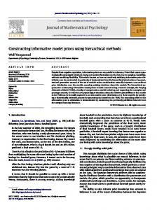
that σ(m) = p0 −−−−−→ · · · pn−1 −−−−−−−→ 1. Composite A state s ∈ CS I of a composite C will be represented by an SDD of |I| variables, each representing the state of an instance i ∈ I. The domain of each variable is determined by the type of the instance. Figure 5 shows this type of encoding for the philosopher example (we consider three philosophers). This encoding reproduces the structure of the IPN specification. We thus find three levels: • The main level describes the states of the three instances p f 1, p f 2 and p f 3 of figure 4. Each instance is represented by one variable. The arcs are labeled using SDD of the PhiloFork level. • The PhiloFork level describes the possible states of a PhiloFork module (see figure 3). The state of a PhiloFork is decomposed into the state of the fork f and the Philo instance p. • The elementary level contains IPN states. For more clarity we have represented left the SDD corresponding to Philo states and right the SDD representing Fork states (see figure 1). These SDD use integer domain variables, and one variable per place of the net. At each level, the possibility of sharing representation is introduced. The labels of the arcs of the upper levels refer to nodes of lower levels. Let us outline in Figure 5 how we can read a state from the structure. In the main SDD, bold gray arcs (labeled with m2) are linked to the m2 entry point in the PhiloFork SDD. Similarly, bold black arcs in the PhiloFork SDD (labeled with f 0) are linked to the f 0

12


«main» level (3 «PhiloFork» modules)

pf1:PF m1 pf2:PF m1

pf2:PF

m3

pf3:PF

pf2:PF

m2

m0

m2

pf3:PF

m0

pf2:PF m3

pf3:PF m2

m3

m1

m3

m2

m0

m1 pf3:PF

m0

1

«PhiloFork» level

m3

m2

f:Fork

m1

f:Fork f1

f0 p:Philo

m0

f:Fork

f:Fork f1

f0

f0 p:Philo

p:Philo p3 p2

p1

f0 p:Philo

p0

«elementary» level

1 p0

p1

p2

p3

f1

HasR

HasR

HasR

HasR

Res

0

1

WaitR

0

WaitR

0 HasL

WaitR

0 HasL

1

1 HasL

0

0 WaitL

WaitL 1

0 Think 1

Think 1

1 WaitR

f0 Res 0

1 1

0

1 WaitL 0

0

one philosopher

one fork

Figure 5. Hierarchical encoding of the full state-space for 3 philosophers

entry in the fork SDD. Finally, double gray arc (labeled with p2) are connected to the p2 entry in the one philosopher SDD. The state where all PhiloFork instances are in state m2 corresponds to a deadlock state: m2 is a state where the fork is not available ( f 0) and the philosopher is in state p2 where WaitR and HasL are marked (he has the left fork and waits for the right one). This example clearly shows that parts of the representation are shared at each level thanks to these relationships between hierarchical levels. For example, the m2 entry of the PhiloFork level is referenced four times in the main level. With “classical” decision diagrams, this type of sharing between parts of the state space could not be achieved.

4.3. Step 3: Transition Encoding: The IPN formalism defines two types: IPN and composite. For each of these concrete realizations of the IPN type contract, we need to define Succ and Locals as homomorphisms.


13

IPN The two following homomorphisms are defined to deal respectively with the pre (noted h− ) and post (noted h+ ) conditions. Both are parameterized by the connected place (p) as well as the valuation (v) labeling the arc entering or outing p . h− (p, v)(ω, s) =  {n−v| n∈s∧n≥v}     ω −−−−−−−−−−−→ Id if ω = p  s    ω→ − h− (p, v) otherwise h− (p, v)(1) = 0

h+ (p, v)(ω, s) =  {n+v| n∈s}     ω −−−−−−−→ Id if ω = p  s    ω→ − h+ (p, v) otherwise

h+ (p, v)(1) = 0

Note that this definition arc by arc of the semantics is well-adapted to the further combination of arcs of different net sub-classes (e.g. inhibitor arcs, reset arcs, capacity places, queues. . . ). Homomorphisms allowing to represent these extensions were previously defined in [12], and are not presented here for sake of simplicity. Locals and Succ are then defined as compositions of these inductive homomorphisms. We use h∈H to denote the composition by ◦ of the homomorphisms h in the set H. Locals =

X

( p∈P h+ (p, Post(p, t)) ◦ h− (p, Pre(p, t)))

t∈T \L

Succ(τ) = p∈P ( t∈τ (h+ (p, Pre(p, t)) ◦ t∈τ (h− (p, Pre(p, t))))) For instance the transition hungry in the model of Fig. 1, would have as homomorphism : hTrans (hungry)h+ (WaitL, 1) ◦ h+ (WaitR, 1) ◦ h− (Idle, 1) When on a path a precondition is unsatisfied, the h− homomorphism will return 0, pruning the path from the structure. Thus the h+ are only applied on the paths such that all preconditions are satisfied. Composite The Next I function is defined using the L homomorphism introduced in section 2.2. For any τ ∈ Bag(T ): M Next I (τ) = i∈I L(i, type(i).Succ(( t)(i))) t∈τ

The homomorphisms representing Locals and Succ , ∀τ ∈ BagT , are encoded: P P Locals = i∈I L(i, type(i).Locals) + t∈S T,V(t)=private NextC.I ({t}) Succ(τ) = NextC.I (τ) To handle synchronization of transitions bearing the same label in different nets of a compositional net definition we use the local application construction of SDD homomorphisms. The fact that this definition as a composition of local actions is possible stems from the simple nature of the synchronization schema considered. A transition relation that is decomposable under this form has been called Kronecker-consistent in various papers on MDD by Ciardo et al like [10]. Figure 2 present a PhiloFork module. The private synchronization getInt of this composite net synchronizes transition p.getL with f.get. This transition corresponds to the philosopher p picking up the fork to his right.

14


The homomorphism encoding this transition getInt is written : Next I ({getInt}) = L(Succ(get), f ) ◦ L(Succ(getL), p) = L(h− (Res, 1), f ) ◦ L(h+ (HasR, 1) ◦ h− (WaitL, 1), p)

4.4. Defining the Verification Goal The last task remaining is to define a set of target (usually undesired) states, and check whether they are reachable, which involves generating the set of reachable states using a fixpoint over the transition relation. The user is then free to define a selection inductive homomorphism that only keeps states that verify an atomic property. This is quite simple, using homomorphisms similar to the pre condition (h− ) that do not modify the states they are applied to. Any boolean combination of atomic properties is easily expressed using union, intersection and set difference. A more complex CTL logic model-checker can then be constructed using nested fixpoint constructions over the transition relation or its reverse [5]. Efficient algorithms to produce witness (counterexample) traces also exist [11] and can be implemented using SDD.

5. Transitive Closure : State of the Art The previous section has allowed us to obtain an encoding of states using SDD and of transitions using homomorphisms. We have concluded with the importance of having an efficient algorithm to obtain the transitive closure or fixpoint of the transition relation over a set of (initial) states, as this procedure is central to the model-checking problem. Such a transitive closure can be obtained using various algorithms, some of which are presented in Algorithm 1. Variant a is a naive algorithm, b [5] and c [19] are algorithms from the literature. Variant d, together with automatic optimizations, is our contribution and will be presented in the next section.

5.1. Symbolic transitive closure (1991) [5] Variation a is adapted from the natural way of writing a fixpoint with explicit data structures: it uses a set todo exclusively containing unexplored states. Notice the slight notation abuse: we note T (todo) when P we should note ( t∈T t)(todo). Variant b instead applies the transition relation to the full set of currently reached states. Variant b is actually much more efficient than variant a in practice. This is due to the fact that the size of DD is not directly linked to the number of states encoded, thus the todo of variant a may actually be much larger in memory. Variant a also requires more computations (to get the difference) which are of limited use to produce the final result. Finally, applying the transition relation to states that have been already explored in b may actually not be very costly due to the existence of a cache. Variant b is similar to the original way of writing a fixpoint as found in [5]. Note that the standard encoding of a transition relation uses a DD with two DD variables (before and after the transition) for each DD variable of the state. Keeping each transition DD isolated induces a high time overhead, as different transitions then cannot share traversal. Thus the union of transitions T is stored as a DD, in other approaches than in SDD. However, simply computing this union T has been shown in some cases to be intractable (leading to more elaborate partitioning algorithms [6]).


15

Algorithm 1: Four variants of a transitive closure loop. Data: {Hom} T : the set of transitions encoded as hT rans homomorphisms S s0 : initial state encoded as an SDD S todo : new states to explore S reach : reachable states a) Explicit reachability style begin todo := s0 reach := s0 while todo , 0 do S tmp := T (todo) todo := tmp \ reach reach := reach + tmp end c) Chaining loop begin todo := s0 reach := 0 while todo , reach do reach := todo for t ∈ T do todo := (t + Id)(todo)

b) Standard symbolic BFS loop begin todo := s0 reach := 0 while todo , reach do reach := todo todo := todo + T (todo) ≡ (T + Id)(todo) end

d) Saturation enabled begin reach := (T + Id)⋆ (s0 ) end

end

5.2. Chaining (1995) [19] An intermediate approach is to use clusters. Transition clusters are defined and a DD representing each cluster is computed using union. This produces smaller DD, that represent the transition relation in parts. The transitive closure is then obtained by algorithm c, where each t represents a cluster. Note that this algorithm no longer explores states in a strict BFS order, as when t2 is applied after t1 , it may discover successors of states obtained by the application of t1 . The clusters are defined in [19] using structural heuristics that rely on the Petri net definition of the model, and try to maximize independence of clusters. This may allow to converge faster than in a or b which will need as many iterations as the state-space is deep. While this variant relies on a heuristic, it has empirically been shown to be much better than b.

5.3. Saturation (2001) [10] Finally the saturation method is empirically an order of magnitude better than c. Saturation consists in constructing clusters based on the highest DD variable that is used by a transition. Any time a DD node of the state space representation is modified by a transition it is (re)saturated, that is the cluster that corresponds to this variable is applied to the node until a fixpoint is reached. When saturating a node, if lower nodes in the data structure are modified they will themselves be (re)saturated. This recursive algorithm can be seen as particular application order of the transition clusters that is adapted to the DD

16


representation of state space, instead of exploring in BFS order the states. The saturation algorithm is not represented in the algorithm variants figure because it is described (in [10]) on a full page that defines complex mutually recursive procedures, and would not fit here. Furthermore, DD packages such as CUDD or Buddy [20, 17] do not provide in their public API the possibility of such fine manipulation of the evaluation procedure, so the algorithm of [10] cannot be easily implemented using those packages.

5.4. Our Contribution All these algorithm variants, including saturation (see [13]), can be implemented using SDD. However we introduce in this paper a more natural way of expressing a fixpoint through the h⋆ unary operator, presented in variant d. The application order of transitions is not specified by the user in this version, leaving it up to the library to decide how to best compute the result. By default, the library will thus apply the most efficient algorithm currently available: saturation. We thus overcome the limits of other DD packages, by implementing saturation inside the library.

6. Automating Saturation This section presents how using simple rewriting rules we automatically create a saturation effect. This allows to embed the complex logic of this algorithm in the library, offering the power of this technique at no additional cost to users. At the heart of this optimization is the property of local invariance.

6.1. Intuition The key idea behind exploiting local invariance is the propagation of operations. Indeed, often operations representing transitions do not affect all variables of the state signature. Thus the homomorphism representing the transition can be propagated, skipping the variables which are not relevant for the transition. This allows to limit the number of (useless) intermediate nodes created during an application of a transition relation. Let us consider the two following homomorphisms leq and inc. leq returns all assignments sequences in which all values of the variable d are less or equal than k, while incd increments all values of d.  {n | n∈s ∧n≤k}     ω −−−−−−−−−−→ Id if ω = x leq(x, k)(ω, s) =  s    ω→ − leq(x, k) else leq(x, k)(1)

= 1  {n+1 | n∈s}     ω −−−−−−−→ Id if ω = x inc(x)(ω, s) =  s    ω→ − inc(x) else inc(x)(1)

= 1

Suppose we have the transition fd = leq(d, 2) ◦ inc(d) to apply on S 1 of the figure 6. We want the full state space, i.e. ( fd + Id)⋆ (S 1 ). A basic BFS application would produce intermediate SDD S 2 to S 4 . However, if the evaluation mechanism could know that variables a, b and c are not relevant for the


+

+

ƒd S1

a {1} b {2} c {3} d {0} 1

17

ƒd S2

a {1} b {2} c {3} d {1} 1

Figure 6.

S3

a {1} b {2} c {3} d {0,1} 1

S4

a {1} b {2} c {3} d {1,2} 1

S5

a {1} b {2} c {3} d {0,1,2} 1

Effects of propagation

operation, we could propagate ( fd + Id)⋆ down to the d node of S 1 , work on that node until the ⋆ fixpoint is reached, then reconstruct the top of the SDD of S 5 . This avoids creation of all the intermediate nodes outlined in grey. The next subsections formalizes this intuition, allowing to embed this logic in the SDD library.

6.2. Local Invariance A minimal structural information is needed for saturation to be possible: the highest variable operations need to be applied to must be known. To this end we define : Definition 6.1. (Locally invariant homomorphism) An homomorphism h is locally invariant on variable ω iff P s − h(δ′ ) ∀δ = hω, π, αi ∈ S, h(δ) = hs,δ′ i∈α ω → Concretely, this means that the application of h doesn’t modify the structure of nodes of variable ω, and h is not modified by traversing these nodes. The variable ω is a “don’t care” w.r.t. operation h, it is neither written nor read by h. A standard DD encoding [10] of h applied to this variable would produce the identity. The identity homomorphism Id is locally invariant on all variables. s For an inductive homomorphism h locally invariant on ω, it means that h(ω, s) = ω → − h. A user defining an inductive homomorphism h should provide a predicate Skip(ω) that returns true if h is locally invariant on variable ω. This minimal information will be used to reorder the application of homomorphisms to produce a saturation effect. It is not difficult when writing an homomorphism to define this Skip predicate since the useful variables are known, it actually reduces the number of tests that need to be written. For example, the h+ and h− homomorphisms of section 4 can exhibit the locality of their effect on the state signature by defining Skip, which removes the test ω = p w.r.t. the previous definition since p is

18


the only variable that is not skipped: {n−v| n∈s∧n≥v}

h− (p, v)(ω, s) = ω −−−−−−−−−−−→ Id h− (p, v).Skip(ω) = (ω , p) h− (p, v)(1) = 0

{n+v| n∈s}

h+ (p, v)(ω, s) = ω −−−−−−−→ Id h+ (p, v).Skip(ω) = (ω , p) h+ (p, v)(1) = 0

An inductive homomorphism φ’s application to δ = hω, π, αi is defined by φ(δ) =

′ hs,δ′ i∈α Φ(ω, s)(δ ). P s − Φ(δ′ ). hs,δ′ i∈α ω →

P

But when Φ is invariant on ω, computation of this union produces the expression This result is known beforehand thanks to the predicate Skip. From an implementation point of view this allows us to create a new node directly by copying the structure of the original node and modifying it in place. Indeed the application of φ will at worst remove some arcs. If a φ(δ′ ) produces the 0 terminal, we prune the arc. Else, if two φ(δ′ ) applications return the same value, we need to fuse the arcs into an arc labeled by the union of the arc values. We thus avoid P computing the expression hs,δ′ i∈α φ(ω, s)(δ), which involves creation of intermediate single arc nodes s

ω→ − · · · and their subsequent union. The impact on the efficiency of this “in place” evaluation is already measurable, but more importantly it enables the next step of rewriting rules.

6.3. Union and Composition For built-in homomorphisms the value of the Skip predicate can be computed by querying their operands: homomorphisms constructed using union, composition and fixpoint of other homomorphisms, are locally invariant on variable ω if their operands are themselves invariant on ω. This property derives from the definition (given in [12, 13]) of the basic set theory operations on DDD and SDD. Indeed for two homomorphisms h and h′ locally invariant on variable ω we have: ∀δ = hω, π, αi ∈ S, (h + h′ )(δ) = h(δ) + h′ (δ) P P s s − h′ (δ′ ) − h(δ′ ) + (s,δ′ )∈α ω → = (s,δ′ )∈α ω → P s − h(δ′ ) + h′ (δ′ ) = (s,δ′ )∈α ω → P s − (h + h′ )(δ′ ) = (s,δ′ )∈α ω → A similar reasoning can be used to prove the property for composition. It allows homomorphisms nested in a union to share traversal of the nodes at the top of the structure as long as they are locally invariant. When they no longer Skip variables, the usual evaluation definition h(δ) + h′ (δ) is used to affect the current node. Until then, the shared traversal implies better time complexity and better memory complexity as they also share cache entries. We further support natively the n-ary union of homomorphisms. This allows to dynamically create clusters by top application level as the union evaluation travels downwards on nodes. When evaluating P an n-ary union H(δ) = i hi (δ) on a node δ = hω, π, αi we partition its operands into F = {hi |hi .Skip(ω)} P P and G = {hi |¬hi .Skip(ω)}. We then rewrite the union H(δ) = ( h∈F h)(δ) + ( h∈G h)(δ), or more simply H(δ) = F(δ) + G(δ). The F union is thus locally invariant on ω and will continue evaluation as a block. P The G part is evaluated using the standard definition G(δ) = h∈G h(δ) Thus the minimal Skip predicate allows us to automatically create clusters of operations by adapting to the structure of the SDD it is applied to. We still have no requirements on the order of variables, as the


19

clusters can be created dynamically. To obtain efficiency, the partitions F + G are cached, as the structure of the SDD typically has limited variation during construction. Thus the partitions for an n-ary union are computed at most once per variable instead of once per node. P The computation using the definition of H(δ) = i hi (δ) requires each hi to separately traverse δ, and forces to fully rebuild all the hi (δ). In contrast, applying a union H allows sharing of traversals of the SDD for its elements, as operations are carried to their application level in clusters before being applied. Thus, when a strict BFS progression (like algorithm 1.b) is required this new evaluation mechanism has a significant effect on performance.

6.4. Fixpoint With the rewriting rule of a union H = F + G we have defined, we can now examine the rewriting of an expression (H + Id)⋆ (δ) as found in algorithm 1.d : (H + Id)⋆ (δ) = (F + G + Id)⋆ (δ) = (G + Id + (F + Id)⋆ )⋆ (δ) The (F + Id)⋆ block by definition is locally invariant on the current variable. Thus it is directly propagated to the successor nodes, where it will recursively be evaluated using the same definition as (H + Id)⋆ . The remaining fixpoint over G homomorphisms can be evaluated using the chaining operation order (see algorithm 1.c), which is reported empirically more effective than other approaches [9], a result also confirmed in our experiments. The chaining application order algorithm 1.c can be written compactly in SDD as : reach = ( t∈T (t + Id))⋆ (s0 ) We thus finally rewrite: (H + Id)⋆ (δ) = ( g∈G (g + Id) ◦ (F + Id)⋆ )⋆ (δ)

6.5. Local Applications We have additional rewriting rules specific to SDD homomorphisms and the L local construction (see section 2.2 ): h(s)

L(h, var)(ω, s) = ω −−−→ Id L(h, var).Skip(ω) = (ω , var) L(h, var)(1) = 0 Note that h is an homomorphism, and its application is thus linear to the values in s. Further a L operation can only affect a single level of the structure (defined by var). We can thus define the following rewriting rules, exploiting the locality of the operation :

20


(1) L(h, v) ◦ L(h′ , v) = L(h ◦ h′ , v) (2) L(h, v) + L(h′ , v) = L(h + h′ , v) (3) v , v′ =⇒ L(h, v) ◦ L(h′ , v′ ) = L(h′ , v′ ) ◦ L(h, v) (4) (L(h, v) + Id)⋆ = L((h + Id)⋆ , v) Expressions (1) and (2) come from the fact that a local operation is locally invariant on all variables except v. Expression (3) asserts commutativity of composition of local operations, when they do not concern the same variable. Indeed, the effect of applying L(h, v) is only to modify the state of variable v, so modifying v then v′ or modifying v′ then v has the same overall effect. Thus two local applications that do not concern the same variable are independent. We exploit this rewriting rule when considering a composition of local to maximize applications of the rule (1), by sorting the composition by application variable. A final rewriting rule (4) is used to allow nested propagation of the fixpoint. It derives directly from rules (1) and (2). With these additional rewriting rules defined, we slightly change the rewriting of (H + Id)⋆ (δ) for node δ = hω, π, αi: we consider H(δ) = F(δ) + L(δ) + G(δ) where F contains the locally invariant part, L = L(l, ω) represents the operations purely local to the current variable ω (if any), and G contains operations which affect the value of ω (and possibly also other variables below). Thanks to rule (4) above, we can write : (H + Id)⋆ (δ) = (F + L + G + Id)⋆ (δ) = (G + Id + (L + Id)⋆ + (F + Id)⋆ )⋆ (δ) = ( g∈G (g + Id) ◦ L((l + Id)⋆ , ω) ◦ (F + Id)⋆ )⋆ (δ) As the next section presenting performance evaluations will show, this saturation style application order heuristically allows to gain an order of magnitude in the size of models that can be treated.

7. Efficiency of Automatic Saturation SDD and automatic saturation have been implemented in the C++ libddd library [18], available under the terms of GNU LGPL. Hereafter reported results were obtained with this library on a Xeon @ 1.83GHz with 4GB of memory. We have run the benchmarks on 4 parametrized models, with different sizes: the well-known Dining Philosophers and Kanban models; a model of the slotted ring protocol; a model of a flexible manufacturing system. We have also benchmarked a LOTOS specification obtained from a true industrial case-study (it was generated automatically from a LOTOS specification – 8,500 lines of LOTOS code + 3,000 lines of C code – by Hubert Garavel from INRIA).

7.1. Impact of Propagation We have first measured on these models how the propagation alone impacts on memory size, that is without automatic saturation. We have thus measured the memory footprint when using a chaining loop with propagation enabled or not. We have observed a gain from 15% to 50%, with an average of about 40%. This is due to the shared traversal of homomorphisms when they are propagated, thus inducing


21

much less creation of intermediary nodes. Although by itself this is a good optimization, automatic saturation allows to gain orders of magnitude in both memory and time.

7.2. Impact of Hierarchy and Automatic Saturation Table 1 shows the results obtained when generating the state spaces of several models with automatic saturation (Algo. 1.d) compared to those obtained using a standard chaining loop (Algo. 1.c). Moreover, we measured how hierarchical encoding of state spaces perform compared to a flat encoding. A such encoding means that we do not use the intrinsic hierarchy of models. Final # Model Size

Hierarchical Chaining Loop Mem. Peak (MB) #

T. (s)

Flat Automatic Sat. Mem. Peak (MB) #

States #

Flat

Hier.

T. (s)

9.8×1021

–

1085

–

LOTOS Specification – – –

–

–

1.47

74.0

1.1×105

100 200 1000 4000

4.9×1062 2.5×10125 9.2×10626 7×102507

2792 5589 27989 –

419 819 4019 16019

1.9 7.9 – –

Dining Philosophers 112 2.8×105 0.2 446 1.1×106 0.7 – – 14 – – –

20 58.1 1108 –

18040 36241 1.8×105 –

0.07 0.2 4.3 77

5.2 10.6 115 1488

4614 9216 46015 1.8×105

10 50 100 150

8.3×1009 1.7×1052 2.6×10105 4.5×10158

1283 29403 – –

105 1345 5145 11445

1.1 – – –

Slotted Ring Protocol 48 90043 0.2 – – 22 – – – – – –

16 1054 – –

31501 2.4×106 – –

0.03 5.1 22 60

3.5 209 816 2466

3743 4.6×105 1.7×106 5.6×106

100 200 300 700

1.7×1019 3.2×1022 2.6×1024 2.8×1028

11419 42819 94219 –

511 1011 1511 3511

12 96 – –

145 563 – –

Kanban 2.6×105 1×106 – –

132 809 2482 –

3.1×105 1.9×106 5.7×106 –

0.4 2.2 7 95

11 37 78 397

14817 46617 1.0×105 5.2×105

50 100 150 300

4.2×1017 2.7×1021 4.8×1023 3.6×1027

8822 32622 71422 –

917 1817 2717 5417

13 – – –

105 627 1875 –

2.2×105 1.3×106 3.8×106 –

0.4 1.9 5.3 33

16 50 105 386

23287 76587 1.6×105 5.9×105

2.9 19 60 –

Flexible Manufacturing System 430 5.3×105 2.7 – – 19 – – 62 – – –

T. (s)

Hierarchical Automatic Sat. Mem. Peak (MB) #

Table 1. Impact of hierarchical decision diagrams and automatic saturation

All “–” entries indicate that the state space’s generation did not finish because of the exhaustion of the computer’s main memory. We have not reported results for flat representation with a chaining loop generation algorithm as they were nearly always unable to handle models of big size. The “Final” grey columns show the final number of decision diagram nodes needed to encode the state spaces for hierarchical and flat encoding. Clearly, flat DD need an order of magnitude of more nodes to store a state space. This shows how well hierarchy factorizes state spaces. The efficiency of hierarchy also show that using a structured specification can help detect similarity of behavior in parts of

22


a model, enabling sharing of their state space representation (see figure 5). But the gains from enabling saturation are even more important than the gains from using hierarchy on this example set. Indeed, saturation allows to mostly overcome the “peak effect” problem. Thus “Flat Automatic Saturation” performs better (in both time and memory) than “Hierarchical Chaining Loop”. As expected, mixing hierarchical encoding and saturation brings the best results: this combination enables the generation of much larger models than other methods on a smaller memory footprint and in less time.

8. Recursive Folding In this section we show how SDD allow us in some cases to gain an order of complexity: we define a solution to the state-space generation of the philosophers problem which has complexity in time and memory logarithmic to the number of philosophers. The philosophers system is highly symmetric, and is thus well-adapted to techniques that exploit this symmetry. We show how SDD allow to capture this symmetry by an adapted hierarchical encoding of the state-space. The crucial idea is to use a recursive “folding” of the model with n levels of depth for 2n philosophers.

8.1. A group of Philosophers We now introduce a composite type definition PhiloForkGroup to represent a group of philosophers (figure 7 left), so that it is identical to a single PhiloFork as defined in figure 3 (from the point of view of the IPN type contract). PhiloForkGroup(2) getL

PhiloRing get

get2 getL

get

getL

pf1:PhiloFork eat

closeGet get

getL

pf2:PhiloFork put

eat

get p:PhiloForkGroup

put

put

eat put closePut

eat2

eat initial = {pf1->initial, pf2->initial}

Figure 7.

initial = {p->initial}

Module containing one Fork and one Philo

We further introduce (figure 7 right) a composite type definition PhiloRing to “close the loop”, and connect the first and last philosophers of a group. These two type definitions can be adapted by setting the type of the instances they contain. In particular, since PhiloFork and PhiloForkGroup have the same transition labels and initial states, one can build a PhiloForkGroup (like in figure 7) that contains instances of (smaller) PhiloForkGroup rather than instances of PhiloFork. Such an encoding can be extremely compact. Suppose the initial state of one PhiloFork is noted (P0 ). The initial state of a PhiloForkGroup(2) is noted M2 = (P0 ) (P0 ). Then the state of PhiloForkGroup(4) is noted M4 = (M2 ) (M2 ). The state of PhiloForkGroup(8) would be M8 = (M4 ) (M4 ), etc... Thus,


23

sharing is extremely high : the initial state of the system for 2n philosophers only requires 2n + k (k ∈ N) nodes to be represented. We can easily adapt this encoding to treat an arbitrary number n of philosophers instead of powers of 2, by decomposing n into it’s binary encoding. For instance, for 5 = 20 + 22 philosophers with a group definition containing a single PhiloFork and a PhiloFrokGroup(4). Such unbalanced depth in the data does not increase computational complexity.

8.2. Experimentations We show in table 2 how SDD provide an elegant solution to the state-space generation of the philosophers problem, for up to 220000 philosophers. The complexity both in time and space is roughly linear to n, with empirically 8n nodes and 12n arcs required to represent the final state-space of 2n philosophers. Nb. Philosophers

States

Time (s)

Final

Peak

210

1.02337×10642

231

1.63233×101346392620

21000 210000 220000

N/A N/A N/A

0.0 0.02 0.81 9.85 20.61

124 282 8034 80034 160034

814 2347 73084 730084 1460084

Table 2. Performance evaluation of recursive folding with 2n philosophers . The states count is noted N/A when the large number library GNU Multiple Precision (GMP) we use reports an overflow.

What is surprising in this problem instance, is that each half of the philosophers at any level actually behaves in the same way as the other half. This is beyond a structural symmetry to global behavioral symmetry. Also when the system is evolving, few system-wide dependencies emerge, the evolution of a Philo depends on its immediate neighbors, not much on people across the table. The solution presented here is specific to the philosophers problem, though it can be adapted to other symmetric problems. Its efficiency here is essentially due to the inherent properties of the model under study. In particular the strong locality, symmetry and the fact that even in a BDD representation, adding philosophers does not increase the “width” of the DDD representation – only it’s height –, are the key factors. The encoding presented here can be used for other very regular systems. However even when such a recursive encoding is possible, logarithmic complexity is not guaranteed. Even when the memory complexity is low, an asymmetry of the initial state may bound optimal complexity to linear (n iterations to pass a token around a ring for instance). Our current research direction consists in defining a translation pattern from higher level notations that express symmetries (e.g. Well-Formed Nets [8]) to IPN. Such a translation could help recognize this pattern and obtain the recursive encoding automatically. In any case, this example reveals that SDD are potentially exponentially more powerful than other decision diagram variants without hierarchy.

24


9. Conclusion In this paper, we have presented the latest evolutions of hierarchical Set Decision Diagrams (SDD), that are suitable to master the complexity of very large systems. We think that such diagrams are well-adapted to process hierarchical high-level specifications such as Net-within-Nets [7] or CO-OPN [2]. We have presented how we optimize evaluation of user operations to automatically produce a saturation effect. Moreover, this automation is done at a low cost for users, since it uses a Skip predicate that is easy to define. We thus generalize the extremely efficient saturation approach of Ciardo et al. [10] by giving a definition that is entirely based on the structure of the decision diagram and the operations encoded, instead of involving a given formalism. Furthermore, the automatic activation of saturation allows users to concentrate on defining the state and transition encoding. We have shown how to build a symbolic model-checker that exploits a hierarchical model definition. To this end we introduced Instantiable Petri Nets, based on a general compositional notion of type and instance. Petri nets were used as elementary component type. Finally, we have shown how recursive folding allows in very efficient and elegant manner to generate state spaces of some regular and symmetric models, with up to 220000 philosophers in our example. Although generalization of this application example is left to further research, it exhibits the potentially exponentially better encoding SDD provide over other DD variants for regular examples. SDD and the optimizations described are implemented in libddd, a C++ library freely available under the terms of GNU LGPL. With growing maturity since the initial prototype developed in 2001 and described in [12], libddd is today a viable alternative to Buddy [17] or CUDD [20] for developers wishing to take advantage of symbolic encodings to build a model-checker.

References [1] Berard, B., Bidoit, M., Finkel, A., Laroussinie, F., Petit, A., Petrucci, L., Schnoebelen, P., McKenzie, P.: Systems and Software Verification: Model Checking Techniques and Tools, chapter Model Checking, Springer Verlag, 2001, 39–46. [2] Biberstein, O., Buchs, D., Guelfi, N.: Object-Oriented Nets with Algebraic Specifications: The CO-OPN/2 Formalism, 2001. [3] Bollig, B., Wegener, I.: Improving the Variable Ordering of OBDDs Is NP-Complete, IEEE Trans. Comput., 45(9), 1996, 993–1002, ISSN 0018-9340. [4] Bryant, R.: Graph-Based Algorithms for Boolean Function Manipulation, IEEE Transactions on Computers, 35(8), August 1986, 677–691. [5] Burch, J., Clarke, E., McMillan, K.: Symbolic Model Checking: 1020 States and Beyond, Information and Computation (Special issue for best papers from LICS90), 98(2), 1992, 153–181. [6] Burch, J. R., Clarke, E. M., Long, D. E.: Symbolic Model Checking with Partitioned Transistion Relations, VLSI, 1991. [7] Cabac, L., Duvigneau, M., Moldt, D., Rölke, H.: Modeling Dynamic Architectures Using Nets-within-Nets, Applications and Theory of Petri Nets 2005, ICATPN 2005, Miami, USA, 3536, 2005. [8] Chiola, G., Dutheillet, C., Franceschinis, G., Haddad, S.: Stochastic Well-Formed Colored Nets and Symmetric Modeling Applications, IEEE Transactions on Computers, 42(11), 1993, 1343–1360.


25

[9] Ciardo, G.: Reachability Set Generation for Petri Nets: Can Brute Force Be Smart?, Applications and Theory of Petri Nets 2004, 2004, 17–34. [10] Ciardo, G., Marmorstein, R., Siminiceanu, R.: Saturation unbound, Tools and algorithms for the construction and analysis of systems, Springer Varlag, LNCS 2619, 2003. [11] Ciardo, G., Siminiceanu, R.: Using Edge-Valued Decision Diagrams for Symbolic Generation of Shortest Paths, FMCAD ’02: Proceedings of the 4th International Conference on Formal Methods in ComputerAided Design, Springer-Verlag, London, UK, 2002, ISBN 3-540-00116-6. [12] Couvreur, J.-M., Encrenaz, E., Paviot-Adet, E., Poitrenaud, D., Wacrenier, P.-A.: Data Decision Diagrams for Petri Net Analysis, ICATPN’02, 2360, Springer-Verlag, 2002. [13] Couvreur, J.-M., Thierry-Mieg, Y.: Hierarchical Decision Diagrams to Exploit Model Structure, Formal Techniques for Networked and Distributed Systems - FORTE 2005, 2005, 443–457. [14] Hamez, A., Thierry-Mieg, Y., Kordon, F.: Hierarchical Set Decision Diagrams and Automatic Saturation, Applications and Theory of Petri Nets 2008, ICATPN 2008, Xian, China, 5062, 2008. [15] Harel, D., Naamad, A.: The STATEMATE Semantics of Statecharts, ACM Trans. Softw. Eng. Methodol., 5(4), 1996, 293–333. [16] Holzmann, G., Smith, M.: A practical method for verifying event-driven software, ICSE ’99: Proceedings of the 21st international conference on Software engineering, IEEE Computer Society Press, Los Alamitos, CA, USA, 1999, ISBN 1-58113-074-0. [17] Lind-Nielsen, J., Mishchenko, A., Behrmann, G., Hulgaard, H., Andersen, H. R., Lichtenberg, J., Larsen, K., Soranzo, N., Bjorner, N., Duret-Lutz, A., Cohen, H. a.: buddy - Library for binary decision diagrams (release 2.4), http://buddy.wiki.sourceforge.net/, 2004. [18] LIP6/Move: the libDDD environment, www.lip6.fr/libddd, 2007. [19] Roig, O., Cortadella, J., Pastor, E.: Verification of asynchronous circuits by BDD-based model checking of Petri nets, 16th International Conference on the Application and Theory of Petri Nets, 815, 1995. [20] Somenzi, F.: CUDD: CU Decision Diagram http://vlsi.colorado.edu/fabio/CUDD/cuddIntro.html, 2005.

Package

(release

2.4.1),

[21] Wang, F.: Formal Verification of Timed Systems: A Survey and Perspective, IEEE, 92(8), August 2004.