Faculty of Electrical Engineering, Mathematics and Computer Science ... The notes provide an introduction into the Finite Element method applied to Partial ...
Building Virtual Models in Engineering An Introduction to Finite Elements Fred Vermolen and Domenico Lahaye Delft University of Technology Faculty of Electrical Engineering, Mathematics and Computer Science Delft Institute for Applied Mathematics November 2011
ii
Preface
Preface to the 2011-2012 Edition In our scientific endeavor we stand upon the shoulder of giants. Early version of these notes were written under the supervision of Frederique le Magnifique and the master himself, who in turn learned the trade from the finite element pioneers at the TU Delft. We thank Niel Budko for pointing to typos in previous versions of these notes, students at the department for their help in further developing the laboratory sessions that make integral part of this course and acknowlegde the help of all the support staff allowing this course to be continued. Domenico Lahaye - 2011 Preface to Earlier Editions These lecture notes are used for the course Finite Elements (WI3098LR) for BSc-students of the department of aerospace engineering with a minor in applied mathematics, and for students visiting the Delft University of Technology in the framework of ATHENS. For the interested student some references are given for further reading, but note that the literature survey is far from complete. The notes provide an introduction into the Finite Element method applied to Partial Differential Equations. The treated problems are classical. The treatment of the Finite Element Method is mathematical, but without the concept of Hilbert and Sobolev spaces, which are fundamental in a rigorous treatment of the Finite Element Method. Recently, a more detailed and comprehensive treatment appeared by van Kan et al. [2006], which is available from the Delft University Press. Further, we recommend all students of this course to attend the lectures since the lecture notes do not aim at being complete. We wish everybody good luck with the material and the course! Further, we would like to thank Caroline van der Lee for the beautiful typesetting of this document. Finally, we thank Fons Daalderop and Martin van Gijzen for their critical reading of these lecture notes and valuable suggestions to improve it. - Alfonzo e Martino, grazie! Fred Vermolen and Domenico Lahaye - 2008 - 2011
iv
Preface
Contents
Preface
iii
1 Introduction 1.1 Stages in a FEM Modeling Procedure . . . . . . 1.2 Motivating Examples . . . . . . . . . . . . . . . . 1.3 Classification of Second Order Partial Differential 1.4 Model Problems . . . . . . . . . . . . . . . . . . 2 Mathematical Preliminaries 2.1 The Geometry of R3 . . . . . . . . . . . . 2.2 Calculus of Functions of a Real Variable . 2.3 Calculus of Functions of Several Variables 2.4 Calculus of Vector Functions . . . . . . .
. . . .
. . . .
. . . .
. . . .
. . . . . . . . . . . . Equations . . . . . .
. . . .
. . . .
. . . .
. . . .
. . . .
3 Minimization Problems and Differential Equations 3.1 Function Spaces, Differential Operators and Functionals . 3.1.1 Function Spaces . . . . . . . . . . . . . . . . . . . 3.1.2 Differential Operators . . . . . . . . . . . . . . . . 3.1.3 Functionals . . . . . . . . . . . . . . . . . . . . . . 3.1.4 Minimization of Functionals . . . . . . . . . . . . . 3.2 Calculus of Variations . . . . . . . . . . . . . . . . . . . . 3.3 From Functionals to Differential Equations . . . . . . . . 3.3.1 Distance in Flat Land . . . . . . . . . . . . . . . . 3.3.2 Abstract One-Dimensional Minimization Problem 3.3.3 Two-Dimensional Self-Adjoint Problem . . . . . . 3.4 From Differential Equation to Minimization Problem . . .
. . . .
. . . . . . . . . . .
. . . .
. . . .
. . . . . . . . . . .
. . . .
. . . .
. . . . . . . . . . .
. . . .
. . . .
. . . . . . . . . . .
. . . .
. . . .
. . . . . . . . . . .
. . . .
. . . .
. . . . . . . . . . .
. . . .
. . . .
. . . . . . . . . . .
. . . .
. . . .
. . . . . . . . . . .
. . . .
. . . .
. . . . . . . . . . .
. . . .
. . . .
. . . . . . . . . . .
. . . .
. . . .
. . . . . . . . . . .
. . . .
. . . .
. . . . . . . . . . .
. . . .
. . . .
. . . . . . . . . . .
. . . .
. . . .
. . . . . . . . . . .
. . . .
1 1 2 4 6
. . . .
9 9 10 10 11
. . . . . . . . . . .
15 15 15 17 17 20 20 21 22 23 26 27
4 Variational Formulation and Differential Equations 29 4.1 Weak forms . . . . . . . . . . . . . . . . . . . . . . . . . . . . . . . . . . . . . . . . . 29 4.2 Which weak formulation? . . . . . . . . . . . . . . . . . . . . . . . . . . . . . . . . . 33 4.3 Mathematical considerations:existence and uniqueness . . . . . . . . . . . . . . . . . 34
5 Galerkin’s Finite Element Method 5.1 The principle of Galerkin’s method . . . . . . . . . . . . . . . . . . . 5.2 Motivation of piecewise linear basis-functions . . . . . . . . . . . . . 5.3 Evaluation of a one-dimensional example . . . . . . . . . . . . . . . . 5.4 Ritz’ method of finite elements by a simple example . . . . . . . . . 5.5 The treatment of a non-homogeneous Dirichlet boundary conditions 5.6 A time-dependent example . . . . . . . . . . . . . . . . . . . . . . . 5.7 The principle of element matrices and vectors . . . . . . . . . . . . . 5.8 Numerical integration . . . . . . . . . . . . . . . . . . . . . . . . . . 5.9 Error considerations . . . . . . . . . . . . . . . . . . . . . . . . . . .
. . . . . . . . .
. . . . . . . . .
. . . . . . . . .
CONTENTS 37 . . . . . . 37 . . . . . . 40 . . . . . . 42 . . . . . . 44 . . . . . . 45 . . . . . . 47 . . . . . . 48 . . . . . . 52 . . . . . . 53
6 Time Dependent Problems: Numerical Methods 6.1 Time-integration methods . . . . . . . . . . . . . . 6.2 Accuracy of time-integration methods . . . . . . . 6.3 Time-integration of PDE’s . . . . . . . . . . . . . . 6.3.1 The heat equation . . . . . . . . . . . . . . 6.3.2 The wave equation . . . . . . . . . . . . . . 6.4 Stability analysis . . . . . . . . . . . . . . . . . . .
. . . . . .
. . . . . .
. . . . . .
. . . . . .
vi
Bibliography
. . . . . .
. . . . . .
. . . . . .
. . . . . .
. . . . . .
. . . . . .
. . . . . .
. . . . . .
. . . . . .
. . . . . .
. . . . . .
. . . . . .
. . . . . .
. . . . . .
. . . . . .
55 55 56 58 59 61 62 65
1 Introduction
In this chapter we aim at • describing five stages that are typical in the application of a finite element method (FEM) modeling procedure for solving engineering problems; • giving examples of how FEM is applied in the modeling of industrial furnaces and electrical energy applications; • giving a list of so-called model problems that will be used in the remainder of this courses.
1.1
Stages in a FEM Modeling Procedure
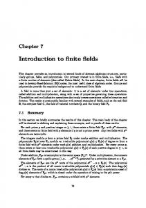
Figure 1.1 shows five different stages in the finite element method (FEM) modeling of the mechanical deformation of a microchip caused by the Ohmic heat generated by an electrical current. The following five stages can be distinguished: • in Stage 1 a geometry model of the device under consideration is build. For this purpose a computer aided design (CAD) software package is typically used; • in Stage 2 the governing physical processes are described in term of appropriate partial differential equations supplied with initial and boundary conditions. In the modeling of electrical energy applications for instances, the Maxwell equations for the electric and magnetic field play a central role; • in Stage 3 the geometry is subdivided into small entities called elements. Different types of mesh generation and mesh refinement techniques exist. General references on this stage are Farrashkhalvat and Miles [2003]; Frey and George [2000]; Liseikin [2010] (mesh generation) and Ainsworth and Oden [2000] (adaptive refinement). Mesh generation techniques are being taught at the TU Delft as part of the Elements of Computational Fluid Dynamics course (WI4011).
2
Introduction
• in Stage 4 the governing partial differential equations are discretized in space and time, a time-stepping procedure is applied to the resulting system of ordinary differential equations and the emerging (non-)linear systems of equations are solved. General references on this stage are Braess [1996]; Eriksson et al. [1996]; Morton and Mayers [1994]; Quarteroni and Valli [1994]; Zienkiewics and Taylor [2000a,b] (general finite elements), Ascher and Petzold [1998] (time-stepping methods), Dennis Jr. and Schnabel [1996]; Kelley [1995] (non-linear system solvers) and Saad [1996]; Smith et al. [1996]; Trottenberg et al. [2001] (linear system solvers). Reference to the mathematical theory underlying the finite element method are for instance Brenner and Scott [2008]; Kreyszig [1989]; Atkinson and Han [2005]. Linear system solvers are being at the TU Delft in the course Scientific Computing (WI4210). TU Delft monographs on ordinary differential equation and on the numerical treatment of partial differential equations are Vuik et al. [2007] and van Kan et al. [2006], respectively. • in Stage 5 the solution of the partial differential equations and derived quantities are visualized on the mesh employed for discretization in space and time. These five stages are typical in any FEM modeling procedure. Although the other stages are not trivial and object of active research, this course mainly focussed on Stage 2 and Stage 4.
Figure 1.1: Stages in a FEM Modeling Procedure.
1.2
Motivating Examples
Industrial Furnace The simulation of flows through an enclosed surface is an often reoccuring problem in computational fluid dynamics. In Figure 1.2 a study case of the simulation of the flow and temperature profile inside an industrial furnace is presented. Fault current limiters Fault current limiters are expected to play an important role in the protection of future power grids. They are capable of preventing fault currents from reaching too high
3
1.2 Motivating Examples
(a) Schematic represention of an industrial furnace
(b) Mesh employed
(c) Simulated temperature profile.
Figure 1.2: Numerical simulation of industrial furnaces.
DC winding AC winding
DC winding AC winding
levels and, therefore enhance the life time expectancy all power system components. Figure 1.3 shows two examples of fault-current limiters along with some finite element simulation results.
(a) Open core configuration
(c) Diffusion coefficient µ Figure 1.3: Numerical simulation of fault current limiters.
(b) Three legged configuration
(d) Current with and without limiter
4
1.3
Introduction
Classification of Second Order Partial Differential Equations
In this section we classify second order linear partial differential equations (PDEs) with constant coefficients according to their elliptic, parabolic and hyperbolic nature and give examples of PDEs in each of these three classes. Classification We consider an open two-dimensional domain (x, y) ∈ Ω ⊂ R2 with boundary Γ = ∂Ω as the domain of the second order linear partial differential equation (PDE) for the unknown field u = u(x, y) and the source function f (x, y) that can be written as L(u) = f on Ω
(1.1)
where the operator L has constant coefficients aij , bi and c L(u) = a11
∂ 2 u(x, y) ∂ 2 u(x, y) ∂u(x, y) ∂u(x, y) ∂ 2 u(x, y) + 2a + a + b1 + b2 + c u(x, y) . (1.2) 12 22 ∂x2 ∂x∂y ∂y 2 ∂x ∂y
We classify these equation based on the sign of the determinant a 11 a12 D= = a11 a22 − a212 . a12 a22
(1.3)
The differential operator L is called • elliptic if D > 0 • parabolic if D = 0 • hyperbolic if D < 0 Prototypes in this classification are the elliptic Laplace equation uxx + uyy = 0, parabolic heat equation uxx − uy = 0 and the hyperbolic wave equation uxx − uyy = 0. In the case of xy-varying coefficients a11 , a22 and a12 , the sign of D and therefore the type of the PDE may change with the location in Ω. As FEM solvers for discretized hyperbolic PDEs are far less developed, we will only consider elliptic and parabolic equations in this course. Elliptic equations are characterized by the fact that changes in the data imposed on the boundary Γ are felt instantaneously in the interior of Ω. Parabolic equations model the evolution of a system from initial to an stationary (time-independent) equilibrium state. Examples of Elliptic Partial Differential Equations We will consider the Poisson equation − 4 u := −
∂ 2 u(x, y) ∂ 2 u(x, y) − =f ∂x2 ∂y 2
(1.4)
as it plays a central role in engineering applications in which the field u solved for plays the role of a (electric, magnetic or gravitational) potential, temperature or displacement. The reason for the minus sign in front of the Laplacian will be discussed together with the finite element
1.3 Classification of Second Order Partial Differential Equations
5
discretization. We will also consider two variants of (1.4). In the first variant we introduce a small positive parameter 0 < � � 1 to arrive at the anisotropic variant −�
∂ 2 u(x, y) ∂ 2 u(x, y) − =f ∂x2 ∂y 2
(1.5)
that can be thought of as a simplified model to study the effect of local mesh refinement required to capture e.g. boundary layers or small geometrical details (such as for instance the air-gap in an electrical machine). In the second variant we again incorporate more physical realism in (1.4) by allowing the parameter c in � � � � ∂ ∂u(x, y) ∂ ∂u(x, y) − c − c =f, (1.6) ∂x ∂x ∂y ∂y to have a jump-discontinuity across the boundary of two subdomains (such as for instance the jump in electrical conductivity across the interface between copper and air). The Helmholtz and the convection-diffusion equation are other examples of elliptic partial differential equations. The former can be written as − 4 u − k2 u = −
∂ 2 u(x, y) ∂ 2 u(x, y) − − k2 u = f , ∂x2 ∂y 2
(1.7)
and models the propagation of an acoustical or electromagnetic wave with wave number k. The latter is a simplified model for the study of a flow with (dimensionless) velocity v = (1, 0) around a body and can be written as −� 4 u + v · ∇u = −�
∂ 2 u(x, y) ∂ 2 u(x, y) ∂u(x, y) − � + =f, ∂x2 ∂y 2 ∂x
(1.8)
where � is the inverse of the Peclet number (which plays the same role as the Reynolds number in the Navier-Stokes equations). The verification that the equations introduced above are indeed elliptic is left as an exercise. The classification given above can be extended to systems of coupled partial differential equations. The vector-valued double curl equation for example relates the vector potential U(x, y, z) = (U1 (x, y, z), U2 (x, y, z), U3 (x, y, z)) with the excitation vector field F(x, y, z) and can be written as ∇ × (ν∇ × U) = F(x, y, z) ,
(1.9)
where as in (1.6) ν represents a material parameter. This model can be derived from the Maxwell equations and plays a central role in the finite element modeling of electrical machines, wind turbines and power transformers. In this setting F and U play the role of the applied current density and the magnetic vector potential, respectively. In order to guarantee uniqueness of the solution of the above elliptic partial differential equations, appropriate (Dirichlet, Neumann or other) boundary conditions on Γ = ∂Ω need to be supplied. Example of a Parabolic Partial Differential Equation In order to give examples of parabolic partial differential equations, we change the notation y into t and consider Ω to be a rectangle (x, t) ∈ Ω = [0, L] × [0, T ]. The parabolic differential equation with source term f (x, t) ∂u(x, t) ∂ 2 u(x, t) = + f (x, t) ∂t ∂x2
(1.10)
6
Introduction
models the diffusion of the quantity u(x, t) in time that reaches a time-independent equilibrium is zero. All of the elliptic models introduced above can be extended to a parabolic state when ∂u(x,t) ∂t model by adding the allowing u to become time-dependent, that is u = u(x, y, t), and adding the term ∂u(x,t) ∂t . These models will be considered for instance when discussing the role of initial vectors of iterative solution methods. In order to guarantee uniqueness of the solution of parabolic partial differential equations, both boundary and initial conditions need to be supplied.
1.4
Model Problems
In this section we define a sequence of model problems for future reference. Elliptic Problem Problems • given the domain x ∈ Ω = (a, b) ⊂ R, given a positive diffusion coefficient c(x) > 0, ∀x ∈ (a, b), and given the boundary data g(x) or h(x), solve for u(x) the following ordinary differential equation d2 u(x) − = f (x) on Ω (1.11) dx2 or � � d du(x) − c(x) = f (x) on Ω (1.12) dx dx supplied with either Dirichlet boundary conditions u(x) = g(x) on x = a and/or x = b
(1.13)
or Neumann boundary conditions d u(x) = h(x) on on x = a and/or x = b . (1.14) dx In case that g(x) = 0 in (1.13) (h(x) = 0 in (1.14)) the Dirichlet (Neumann) boundary conditions is called homogeneous. • given an open and bounded domain (x, y) ∈ Ω ⊂ R2 with bounded by a close curve Γ = ∂Ω that can be subdivided as Γ = ΓD ∪ ΓN and has outward normal n, given a positive diffusion coefficient c(x, y) > 0, ∀(x, y) ∈ Ω, and given the boundary data g(x, y) or h(x, y), solve for u(x, y) the following partial differential equation ∂ 2 u(x, y) ∂ 2 u(x, y) − = f (x, y) on Ω , ∂x2 ∂y 2 or � � � � ∂ ∂u(x, y) ∂ ∂u(x, y) − c(x, y) − c(x, y) = f (x, y) on Ω , ∂x ∂x ∂y ∂y supplied with either Dirichlet boundary conditions − 4 u := −
(1.15)
(1.16)
u(x, y) = g(x, y) on ΓD
(1.17)
∂u(x, y) = ∇u(x, y) · n = h(x, y) on ΓN . ∂n
(1.18)
or Neumann boundary conditions
7
1.4 Model Problems
• given an open and bounded domain (x, y, z) ∈ Ω ⊂ R3 bounded by a closed surface S = ∂Ω that can be subdivided into S = SS ∪SN and has outward normal n, given a positive coefficient ν(x, y, z) > 0, ∀(x, y, z) ∈ Ω, given a source function F(x, y, z) and given the boundary data G(x, y, z) or H(x, y, z), solve for U (x, y, z) the following partial differential ∇ × (ν∇ × U) = F(x, y, z) ,
(1.19)
supplied with either Dirichlet boundary conditions U(x, y, z) = G(x, y, z) on SD ,
(1.20)
or conditions on the tangential derivatives of U (∇ × U) × n = G(x, y, z) on SN .
(1.21)
Parabolic Model Problems • given the domain x ∈ Ω = (a, b) ⊂ R and the time time interval t ∈ [0, T ], given a positive diffusion coefficient c(x) > 0, ∀x ∈ (a, b), given initial conditions u0 (x) = u(x, t = 0) and given the boundary data g(x) or h(x), solve for u(x, t) the following partial differential equation � � ∂ ∂u(x, t) ∂u(x, t) = c(x) + f (x) on Ω × [0, T ] (1.22) ∂t ∂x ∂x supplied with either Dirichlet boundary conditions u(x, t) = g(x) on x = a and/or x = b
∀t ∈ [0, T ]
(1.23)
or Neumann boundary conditions ∂ u(x, t) = h(x) on on x = a and/or x = b ∂x
∀t ∈ [0, T ]
(1.24)
and the initial condition u(x, t = 0) = u0 (x)
∀x ∈ Ω .
(1.25)
8
Introduction
2 Mathematical Preliminaries
The goals and motivations of this chapter are to • generalize the concept of a primitive of a scalar function in a single real variable to vectorvalued functions resulting in the concept of a (scalar or vector) potential; • generalize the integration by parts formula for integrals of scalar functions to integrals of vector-valued functions allowing to cast the strong form of a partial differential equation problem into its weak (or variational) form; • give the fundamental lemma of variational calculus as allowing to demonstrate the equivalence of the strong and weak form of a partial differential equation problem. We refer to Stuart for details.
2.1
The Geometry of R3
We denote a point in the three-dimensional Euclidean space R3 by x = (x, y, z). We denote a vector u in R3 either by its components (u1 , u2 , u3 ) or by the (vectorial) sum of the components times the respective unit vectors in x, y and z-direction, .i.e, u = u1 i + u2 j + u3 k. Inner product and norm We denote the inner product (or scalar product) of two vectors u = (u1 , u2 , u3 ) and v = (v1 , v2 , v3 ) in R3 by u · v. The result of this product is a number (or scalar) defined as u · v = u1 v1 + u2 v2 + u3 v3 . (2.1) The norm of the vector u denoted as kuk is defined as kuk =
√
u·u=
√
u1 u1 + u2 u2 + u3 u3 .
(2.2)
10
Mathematical Preliminaries
Outer product We denote and v = (v1 , v2 , v3 ) in R3 by i j u × v = u1 u2 v1 v2
the outer product (or vector product) of two vectors u = (u1 , u2 , u3 ) u × v. The result of this product is a vector defined as k (2.3) u3 = [u2 v3 − u3 v2 ] i − [u1 v3 − u3 v1 ] j + [u1 v2 − u2 v1 ] k . v3
The triple product of three vectors u, v and w is defined as (u × v) · w and satisfies (u × v) · w = u · (v × w)
2.2
(2.4)
Calculus of Functions of a Real Variable
Assume f (x) to be a scalar function in a single real variable x. A point x0 in the domain of f such that ddxf (x = x0 ) = f 0 (x0 ) = 0 is called a critical point of f (x). The function f (x) attains its (local) minima and maxima in its first order critical points (though not all first order critical points are minima or maxima of f (x)). The Fundamental theorem of Calculus states that, given a function Rb f (x) in a single real variables with primitive F (x), the integral a f (x) dx can be computed as Z
b
f (x) dx = F (b) − F (a) .
(2.5)
a
The following integration by parts formula holds Z b Z b b 0 f (x) g (x) dx = [f (x)g(x)]a − f 0 (x) g(x) dx . a
2.3
(2.6)
a
Calculus of Functions of Several Variables
Assume u(x) = u(x, y, z) to be be a function on R3 , i.e., u(x) : R3 7→ R. Assume furthermore x0 to be point in the domain of u(x) and s a unit vector, respectively. Directional Derivative The derivative of u(x) in the direction s in the point x0 is denoted as Ds u(x0 ) and defined as u(x0 + � s) − u(x0 ) d = [u(x0 + � s)] |�=0 . �→0 � d�
Ds u(x0 ) = lim
(2.7)
This derivative gives the rate of change u(x) = u(x, y, z) in the direction of s at the point x0 . Gradient The gradient of u denoted as grad u = ∇u is vector function that is defined as � � ∂u ∂u ∂u ∂u ∂u ∂u ∇u = , , = i+ j+ k = ux i + uy j + uz k . ∂x ∂y ∂z ∂x ∂y ∂z
(2.8)
The gradient of u is allows to compute the directional derivative of u in the direction of s. We indeed have that Ds u(x0 ) = ∇u(x0 ) · s. This identity will be useful in formulating necessary conditions for first order critical points of u(x). In a physical context and in case that u is e.g. the temperature, ∇u is proportional to the heat flux.
11
2.4 Calculus of Vector Functions
First Order Critical Points The point x0 is a first order critical point of u(x0 ) iff ∇u(x0 ) = 0 in R3 . The latter condition can be stated equivalently as d [u(x0 + � s)] |�=0 = 0 ( in R) ∀s ∈ R3 with ksk = 1 . (2.9) d� This condition will be allow to define first order critical point of functionals on infinite dimensional vector spaces in the next chapter.
2.4
Calculus of Vector Functions
Assume F(x) = (F1 (x), F2 (x), F3 (x)) to be a vector function on R3 , i.e., F(x) : R3 7→ R3 . Divergence and curl The divergence of F denoted as div F = ∇ · F is a scalar function that is defined as ∂F1 ∂F2 ∂F3 + + . (2.10) ∇·F= ∂x ∂y ∂z The curl (or rotation) of F denoted as curl F = ∇ × F is a vector function that is defined as ∂F ∂F2 3 � � � � � � ∂y − ∂z ∂F3 ∂F2 ∂F3 ∂F1 ∂F2 ∂F1 ∂F3 ∂F1 ∇ × F = − ∂x + ∂z = − i− − j+ − k. (2.11) ∂y ∂z ∂x ∂z ∂x ∂y ∂F1 ∂F2 ∂x − ∂y The divergence of the vector field F evaluated at a particular point x is the extent to which the vector field behaves like a source or a sink at a given point. If the divergence is nonzero at some point then there must be a source or sink at that position. The curl of a vector field F describes an infinitesimal rotation of F. Example 2.4.1. Insert examples as in previous version of the ATHENS notes here. Example 2.4.2. Assume c(x) and u(x) to be two scalar functions. Then c ∇u is a vector function whose divergence is equal to � � � � � � ∂ ∂u ∂ ∂u ∂ ∂u ∇ · (c ∇u) = c + c + c . (2.12) ∂x ∂x ∂y ∂y ∂z ∂z If in particular c = 1 (i.e. c(x) = 1 for all x), then ∇ · ∇u = 4φ =
∂2u ∂2u ∂2u + + , ∂x2 ∂y 2 ∂z 2
(2.13)
where 4u denotes the Laplacian of u. This differential operator is generalized to vector-valued functions F(x) by the double-curl operator as ∇ × (c∇ × F). Proposition 2.4.1. From the above definitions immediately follows that for any scalar function u and for any vector function F that ∇ × (∇u) = 0 (in R3 )
(2.14)
∇ · (∇ × F) = 0 (in R) .
(2.15)
We will see below that scalar functions u that satisfy ∇ · u = 0 and vector functions F that satisfy ∇ × F = 0 play a special role as they generalize the notion of a constant function f (x) for which f 0 (x) = 0.
12
Mathematical Preliminaries
Proposition 2.4.2. Let c, u and v be scalar functions and let F, G and U be vector functions. By applying the product rule for differentiation, the following properties can be derived ∇ · (vF) = v∇ · F + ∇v · F
(2.16)
∇ · (F × G) = (∇ × F) · G + (∇ × G) · F .
(2.17)
Setting in the former equality F = c (∇u), yields ∇ · [(c ∇u)v] = [∇ · (c ∇u)] v + c ∇u · ∇v .
(2.18)
while putting in the latter equality F = c (∇ × U), yields ∇ · [c (∇ × U) × G] = [∇ × (c∇ × U)] · G + (∇ × G) · (c∇ × U) .
(2.19)
Flux and first integration theorem Assume S to be an oriented surface in R3 with unit outward normal n. We will denote by −S the surface that coincides with S and has opposite orientation. The normal derivative on S of the function u denoted as un is defined as un = ∇u · n. The flux of F through S denoted as Φ is defined as the surface integral Z Z Φ= F · dS = F · n dS . (2.20) S
S
Assume the surface S to be closed and enclosing a volume V . We make this relation explicit by writing S = S(V ). The Gauss integration theorem states that Z Z F · dS = ∇ · F dV . (2.21) S(V )
V
Proposition 2.4.3. Assume as in Proposition 2.4.2 c, u and v to be scalar functions and F, G and U to be vector functions. Applying Gauss’ Theorem to the vector function v F and using (2.16) to expand the right-hand side yields Z Z Z Z F v · dS = ∇ · [F v] dV = v∇ · F dV + ∇v · F dV . (2.22) S(V )
V
V
V
Setting F = c (∇u) yields Z Z Z [c (∇u)] v · dS = v∇ · [c (∇u)] dV + ∇v · [c (∇u)] dV . S(V )
V
(2.23)
V
Using the notation un = ∇u · n for the normal derivative, one can write the integrand in the lefthand side as [c (∇u)] v · dS = [c (∇u)] v · n dS = c un v dS. After rearranging terms, we obtain the following integration by parts formula Z Z Z [∇ · (c ∇u)] v dV = c un v dS − c ∇u · ∇v dV . (2.24) V
S(V )
V
Applying Gauss’ Theorem to the vector function F × G and using (2.17) to expand the right-hand side yields Z Z Z Z F × G · dS = ∇ · (F × G) dV = (∇ × F) · G dV + (∇ × G) · F dV . (2.25) S(V )
V
V
V
13
2.4 Calculus of Vector Functions
We use the identify (2.4) to rewrite the integrand in the left-hand side as F×G·dS = (F×G)·n dS = F · (G × n) dS. Setting F = c (∇ × U) and rearranging terms then yields Z Z Z c (∇ × U) · (G × n) dS − (c ∇ × U) · (∇ × G) dV . (2.26) [∇ × (c ∇ × U)] · G dV = V
S(V )
V
In subsequent chapters, we will extensively use a two-dimensional variant of (2.24) in which an oriented surface Ω with outward normal n in R2 (that later we will later call a computational domain) is bounded by a boundary Γ = ∂Ω. In this case we the following integration by parts formula Z Z Z c ∇u · ∇v dΩ ,
c un v dΓ −
[∇ · (c ∇u)] v dΩ =
(2.27)
Ω
Γ(Ω)
Ω
Divergence-Free Vector Fields and Existence of Vector Potentials A vector function F is called divergence-free (or solenoidal) on Ω ⊂ R3 if and only if ∇ · F(x) = 0 (in R) for all x ∈ Ω. Unless stated differently, we will call in these notes a vector function F divergence-free if and only if it is divergence-free on Ω = R3 . Gauss’ theorem implies that the flux of a divergence-free vector field through a closed surface S is zero. Decomposing S as S = S + + (−S − ), the flux of a divergence-free F through S + and S − can then be seen to be equal. Given that S was chosen arbitrarily, the flux of a divergence-free vector in surface independent. This surface-independent property allows in turn to demonstrate that for divergence-free vector fields a vector potential A must exist such that F=∇×A , or component-wise � � � � � � ∂A3 ∂A2 ∂A3 ∂A1 ∂A2 ∂A1 F1 = − , F2 = − + and F3 = − . ∂y ∂z ∂x ∂z ∂x ∂y
(2.28)
(2.29)
Circulation and second integration theorem Assume Γ to be a closed oriented curve in R3 with unit tangential vector t. We will denote by −Γ the curve that coincides with Γ and has opposite orientation. The tangential derivative along Γ of the function u denoted as ut is defined as ut = ∇u · t. The circulation of F along Γ denoted as C is defined as the line integral Z Z C= F · dΓ = F · t dΓ . (2.30) Γ
Γ
Assume that the curve Γ encloses a surface S and that this relation in written as Γ(S). The Stokes’ integration theorem states that Z Z F · dΓ = (∇ × F) · dS . (2.31) Γ(S)
S
Curl-Free Vector Fields and Existence of Scalar Potentials A vector function F is called curlfree (or irrotational) on Ω ⊂ R3 if and only if ∇ × F(x) = 0(in R3 ) for all x ∈ Ω. Unless stated differently, we will call in these notes a vector function F curl-free if and only if it is curl-free on Ω = R3 .
14
Mathematical Preliminaries
Stokes’ theorem implies that the circulation of a curl-free vector field along a closed curve Γ is zero. Decomposing Γ as Γ = Γ+ + (−Γ− ), the line integral of a divergence-free F along Γ+ and Γ− can then be seen to be equal. Given that Γ was chosen arbitrarily, the circulation of a curl-free vector is path independent. This path-independent property allows in turn to demonstrate that for curl-free vector fields a scalar potential u must exist such that F=∇·u ,
(2.32)
or component-wise F1 =
∂u ∂u ∂u , F2 = and F3 = . ∂x ∂y ∂z
(2.33)
3 Minimization Problems and Differential Equations
A physical system evolves in such a way to minimize their internal energy. Newton’s apple falls due to gravitation. The thermal or magnetic flux passes by preference through regions of high (thermal or magnetic) conductivity. Partial differential equations are derived from this principle. Instead of solving the differential problem directly it might therefore be more advantegeous to consider an equivalent energy minimization problem. In this chapter we put the equivalence between partial differential equations and minimization problems in a more formal setting as it will serve as a tool to explain FEM to solve the former. In this chapter we aim at [1] give the fundamental lemma of variational calculus known as du Bois-Reymond’s lemma; [2] derive the Euler-Lagrange equation whose solution describes a stationary point for a functional to be minimized; [3] use the above two ingredients to show how partial differential equations can be derived from a minimization problem; [4] show under which conditions a partial differential differential can be derived from a minimization problem.
3.1
Function Spaces, Differential Operators and Functionals
In this section we introduce ingredients allowing to describe minimization problems formally. We seek to describe that the orbit that the falling apple describes is an orbit that minimizes its energy. 3.1.1
Function Spaces
In the following we will denote Ω as open and bounded domain in R, R2 or R3 that we will refer to as the computational domain. As Ω is open, it does not contain its boundary. The union of Ω
16
Minimization Problems and Differential Equations
and its boundary is called the closure of Ω and denoted as Ω. We recall that a space V is a vector space iff V is closed for linear combinations, iff c1 , c2 ∈ R and v1 , v2 ∈ V implies that c1 v1 + c2 v2 ∈ V . Definition 3.1.1. (Function space) Given an open and bounded domain Ω (in R, R2 or R3 ), a function space V (Ω) is a vector space of functions (in one, two or three variables) on Ω that satisfy some smoothness requirements and possibly boundary conditions. The set V (Ω) is e.g. the set of all imaginable orbits of the Newton’s apple. We impose sufficient smoothness conditions to allow to take derivatives of elements in V (Ω). If additionally boundary conditions are imposed, elements V (Ω) can be viewed as solutions of a partial differential equation supplied with boundary conditions. More formally, we can give the following examples: Example 3.1.1. (One-Dimensional Domain) Given the open interval Ω = (a, b) ⊂ R, we will Rb denote by L2 (Ω) the set of square integrable functions on Ω, i.e., u ∈ L2 (Ω) iff a u2 (x) dx < ∞ and by H 1 (Ω) the set of square integrable function with square integrable first derivative, i.e, u ∈ H 1 (Ω) �2 Rb Rb iff a u2 (x) dx < ∞ and a du dx < ∞. Clearly H 1 (Ω) ⊂ L2 (Ω). We will denote by C (Ω) the dx function that are continuous on Ω. If u ∈ C (Ω), than u is bounded (as continuous function function on a compact set) and therefore square integrable, i.e., C (Ω) ⊂ L2 (Ω). We will denote by C 1 (Ω) and C 2 (Ω) the functions u(x) with a continuous first derivative u0 (x) and continuous second derivative u00 (x) on Ω , respectively. Assume that x0 ∈ (a, b) and δ > 0 such that both x−δ = x0 − δ ∈ (a, b) and xδ = x0 + δ ∈ (a, b). We define the functions v1 (x), v2 (x) and v3 (x) as piecewise constant, linear and quadratic polynomials follows ( 0 if |x − x−δ | > δ v1 (x) = (3.1) 1 if |x − x−δ | ≤ δ 0 if |x − x−δ | > δ v2 (x) = (3.2) (x − x−δ )/(x0 − x−δ ) if x−δ ≤ x ≤ x0 (xδ − x)/(xδ − x0 ) if x0 ≤ x ≤ xδ 0 if |x − x−δ | > δ v3 (x) = (3.3) (x − x−δ )2 /(x0 − x−δ )2 if x−δ ≤ x ≤ x0 2 2 (xδ − x) /(xδ − x0 ) if x0 ≤ x ≤ xδ Then v1 (x) has a jump discontinuity in both x = x−δ and x = xδ , and therefore v1 (x) ∈ / C (Ω). The function v2 (x) is continuous, but its derivative has a jump discontinuity in x = x−δ , x = x0 and x = xδ , and therefore v2 (x) ∈ C (Ω) \ C 1 (Ω). The function v3 (x) is continuous and has a continuous first derivative, but its second derivative has a jump discontinuity in x = x−δ , x = x0 and x = xδ , and therefore v3 (x) ∈ C 1 (Ω) \ C 2 (Ω). The function v2 (x) is informly referred to as the hat-function, and will play a central role in the application of the FEM method. We denote the subset C0 (Ω) = {u ∈ C (Ω) | u(a) = 0 = u(b)} of functions satisfying homogeneous Dirichlet boundary conditions. The space C01 (Ω) and C02 (Ω) are defined similarly. Example 3.1.2. (Two-Dimensional Domain) In problems on two-dimensional domain, we will denote by Ω ⊂ R2 an open and bounded domain with boundary Γ = ∂Ω that can be partioned into distinct parts ΓD and ΓN , i.e., Γ = ΓD ∪ΓN . We associate with ΓD and ΓN that part of the boundary on which (possibly non-homogeneous) Dirichlet and Neumann (or Robin) boundary conditions are
17
3.1 Function Spaces, Differential Operators and Functionals
imposed, respectively. We will denote by C 1 (Ω) the functions u(x,�y) with a continuous first order 1 1 partial derivatives ux and uy . We will denote the subset C0 (Ω) = u ∈ C (Ω) | u|ΓD = 0 . Treatment of boundary conditions The presence of the Neumann boundary conditions is not reflected in the above definition of C01 (Ω). The condition u|ΓD = 0 is imposed even in case of non-homogenous Dirichlet boundary conditions. Only with the latter condition the above function spaces are vector space (closed for linear combinations) of infinite dimensions. These vector spaces can be endowed with a inner-product, thus becoming therefore Hilbert spaces. 3.1.2
Differential Operators
Assume that L is a second order differential operator acting on elements of V (Ω) and let u = 0, i.e., u(x) = 0 ∀x ∈ Ω, denote the zero element of V (Ω). It is obvious that Lu = 0. This trivial situation is excluded in the following definition. Definition 3.1.2. (Positivity) The differential operatore L is positive on V (Ω) iff Z v (Lv) dΩ > 0 ∀v ∈ V (Ω) \ {0} .
(3.4)
Ω
Observe that in the above definition the boundary conditions are taken into account by incorporating in the definition of V (Ω) and requiring that v ∈ V (Ω). 2
d v 00 1 Example 3.1.3. The differential operator Lv = − dx 2 = −v (x) is positive on C0 ((a, b)). Indeed, using integration by parts and the homogeneous Dirichtlet boundary conditions we have that
Z
Z v (Lv) dΩ = −
Ω
a
b
� �b v(x) v (x) dx = − v(x) v 0 (x) a + | {z } 00
Z
b
v 0 (x) v 0 (x) dx > 0 .
(3.5)
a
=0
Example 3.1.4. Given on open and bounded subset Ω ⊂ R2 and the coefficient c(x) > 0 ∀x ∈ Ω, the differential operator Lv = −∇ · (c∇v) is positive on C01 (Ω). Definition 3.1.3. (Self-adjointness) The differential operator L is called self-adjoint (or symmetric) on V (Ω) iff Z Z v (Lu) dΩ = u (Lv) dΩ ∀u, v ∈ V (Ω) . (3.6) Ω
Ω 2
d v 1 Example 3.1.5. The differential operator Lv = − dx 2 is self-adjoint on C0 ((a, b)). This can be seen by integrating by parts twice and using the homogeneous boundary conditions.
Example 3.1.6. Given an open and bounded subset Ω ⊂ R2 and the coefficient c(x) > 0 ∀x ∈ Ω, the differential operator Lv = −∇ · (c∇v) is self-adjoint on C01 (Ω). 3.1.3
Functionals
Definition 3.1.4. (Functional) Given a function space V (Ω), a functional L is a mapping from V (Ω) onto R, i.e., L : V (Ω) 7→ R.
18
Minimization Problems and Differential Equations
If u ∈ V (Ω) is an orbits of Newton’s apple, then L(u) can for instance represent the length of the orbit. If u ∈ V (Ω) is a temperature distribution in a region, then can for instance represent the average of the temperature. In the modeling of electrical machines the function u typically represents the (scalar or vector) magnetic potential and the force, torque, resistive heat and eddy current are examples of functionals in u. More formal examples are given below. Example 3.1.7. (Distance in Flat Land) Let V (Ω) be the set of differentiable functions on the open interval (a, b) supplied with the additional conditions that u(x = a) = ua and u(x = b) = ub . The graph of each element of V (Ω) is a path between the points (a, ua ) and (b, ub ) in R2 . The length L(u) of each of these path can be computed by the line integral Z L(u) = ds (3.7) where, given that dy = u0 (x) dx, p � � ds2 = dx2 + dy 2 = 1 + u0 (x)2 dx2 ⇔ ds = 1 + u0 (x)2 dx ,
(3.8)
Z bp L(u) = 1 + u0 (x)2 dx .
(3.9)
and therefore a
Example 3.1.8. (Mass-Spring System) Let V (Ω) be the set of differentiable functions on the open interval (a, b) describing the motion of a point (apple) with mass m vertically attached to a wall with a spring constant k (the independent variable x ∈ (a, b) thus denotes time here). The instantaneous energy E [u(x)] of the mass is the sum of the kinetic and potential energy T [u(x)] = 1/2 m u0 (x)2 and V [u(x)] = 1/2 k u(x)2 , i.e, E [u(x)] = T [u(x)] − V [u(x)]. The total energy is the functional L(u) defined on V (Ω) as Z L(u) =
b�
� T [u(x)] − V [u(x)] dx =
a
Z
b�
1/2 m u0 (x)2
� − 1/2 k u(x)2 dx .
(3.10)
a
Example 3.1.9. (Abstract One-Dimensional Example) The previous example can be put in a more abstract setting by allowing f (x, u, u0 ) to be a function in three variables mapping from (a, b) × V (Ω) × V (Ω) to R with sufficiently smooth partial derivatives. Given such a function f , we define the functional on V (Ω) as Z L(u) =
b
f (x, u, u0 ) dx .
(3.11)
a
In the next example we establish the link we differential equations. In this example the function f represents the source term in the differential equation, the current in the modeling of fault-current limiter or the burner in the industrial furnace example. The function c and h will turn out later to be the diffusion coefficient and the non-homogeneous term in the Neumann boundary conditions, respectively. Example 3.1.10. (Two-Dimensional Self-Adjoint Differential Equation) Given Ω ⊂ R2 an open and bounded two-dimensional domain with boundary Γ = ΓD ∪ ΓN , given c a positive function
3.1 Function Spaces, Differential Operators and Functionals
Figure 3.1: A smooth curve in R2 that connects the points (a, ua ) and (b, ub )
19
20
Minimization Problems and Differential Equations
on Ω, given f a continuous function on Ω and given h a function on ΓN , a functional on C 1 (Ω) can be defined by � Z � Z 1/2 ∇u · (c∇u) − f u dΩ + L(u) = h(x, y) u dΓ . (3.12) Ω
ΓN
In turns out in the last example L is linear and bounded (and therefore continuous). 3.1.4
Minimization of Functionals
In this subsection we seek to minimize functionals over the corresponding function space, i.e., to find arguments u ˜ ∈ V (Ω) that minimize L or find u ˜ ∈ V (Ω) such that L(˜ u) ≤ L(u) ∀u ∈ V (Ω) .
(3.13)
Solving this problem is generally hard, if not impossible at all. Local and global minimizers might be hard to distinguish and the global optimum might be non-unique. We therefore aim towards the less ambitious goal of seeking first order critical points of L. These points are defined for functionals in the same way as for functions in several variables. The point u ˜ is a first order critical point of L iff the directional derivative of L in u ˜ is zero in all possible directions. For the definition of first order critical point to have sense, it is important that the space of possible directions used in the definition forms a vector space, i.e., that this space is closed for linear combinations. This requires the proper treatment of the non-homogeneous Dirichlet boundary conditions. Indeed, any linear combination of two functions u1 and u2 satisfying the nonhomogeneous Dirichlet boundary conditions no longer satisfies them. This motivates the following definition of the subspace V0 (Ω) of V (Ω) V0 (Ω) = {v ∈ V (Ω)|v|ΓD = 0} .
(3.14)
In case that non-homogeneous Dirichlet boundary conditions are imposed the space V0 (Ω) forms a vector space, while V (Ω) does not. The problem of finding (local) minimizers of L now reduces to find u ˜ ∈ V (Ω) such that
� d� L(˜ u + �v) |�=0 = 0 ∀v ∈ V0 (Ω) . d�
(3.15)
Note that u ˜ and v not necessarily belong to the same space. We will refer to V0 (Ω) as the space of test functions. Only if L is convex, there is only one critical point that coincides in the global minimizer of L.
3.2
Calculus of Variations
For future reference we recall here a classical result from variational calculus, which we will refer to as the du Bois-Reymond Lemma (after Paul David Gustav du Bois-Reymond (Germany, 1831 1889) (details can be found in e.g. the monographs van Kan et al. [2006]; Strang and Fix [1973]). Lemma 3.2.1. (One-dimensional du Bois-Reymond’s Lemma) Assume Ω = (a, b) and let V0 (Ω) denote a function space of sufficiently smooth function on Ω that vanish on the boundary of
21
3.3 From Functionals to Differential Equations
Ω. Assume f (x) be continuous over Ω, i.e., f ∈ C(Ω) and suppose that Zb ∀v ∈ V0 (Ω) .
f (x) v(x) dx = 0,
(3.16)
a
Then f (x) = 0 on Ω.
(3.17)
The equality (3.19) states that f (x) is zero in variational or weak form, while (3.20) states that f (x) is zero is strong form. Two functions f (x) and g(x) as said to be equal in weak form if their difference is zero in weak from. The lemma states that for continuous functions the notion on weak and strong form of being zero on interior of the domain Ω coincide. No information on the behavior of f (x) on the boundary of Ω is deduced. In this context the space V0 (Ω) is called the space of test functions. The practical value of this lemma increases as the space V0 (Ω) can be kept small, in such a way to require to test with as few as function v ∈ V0 (Ω) as possible. Indeed, if the lemma holds for a given V0 (Ω) it will automatically be valid for a larger space Z0 (Ω) (as a subset of test functions v ∈ V0 (Ω) ⊂ Z0 (Ω) already suffices to draw the conclusion). Proof. We will prove the lemma for V0 (Ω) = C01 (Ω) (and therefore by the previous argument also for V0 (Ω) = C0 (Ω)). We argue by contradiction. Suppose that f (x0 ) > 0 for any x0 ∈ (a, b) (note that the case f (x0 ) < 0 can be treated similarly) then since f (x) is continuous, there exists a δ > 0 such that f (x) > 0 whenever |x − x0 | < δ. Now we choose v(x) = v3 (x) defined by Equation 3.3. Then v(x) ∈ C01 (Ω), v(x) > 0 on (x0 −δ, x0 +δ) and xZ0 +δ Zb f (x) v(x) dx = f (x) v(x) dx > 0. (3.18) |{z} |{z} a
x0 −δ
>0
>0
This violates the hypothesis (3.19). As x0 was chosen arbitrarily, we have proven that f (x) = 0 on Ω. � The du Bois-Reymond’s Lemma also holds in higher dimensions. Lemma 3.2.2. (Higher-dimensional du Bois-Reymond’s Lemma) Assume Ω to be an open and bounded domain in R2 and let V0 (Ω) denote a function space of sufficiently smooth function on Ω that vanish on the boundary of Ω. Assume f (x, y) be continuous over Ω, i.e., f ∈ C(Ω) and suppose that Z f (x, y) v(x, y) dΩ = 0,
∀v ∈ V0 (Ω) .
(3.19)
Ω
Then f (x, y) = 0 on Ω.
3.3
(3.20)
From Functionals to Differential Equations
In this section we illustrate how differential equations can be obtained by the minimizing of functionals. Given a functional L, we will carry out the following three-step procedure:
22
Minimization Problems and Differential Equations
[1] assume that u ˜ is a first-order critical point of L and express that u ˜ satisfies the condition (3.15); [2] integrate integrate-by-parts and exploit the homogeneous Dirichlet boundary conditions of v ∈ V0 (Ω); [3] apply du-Bois Reymond’s Lemma to derive the differential equation for u ˜ supplied with boundary conditions. In what follows we illustrate the above procedure using the examples of functionals given above. 3.3.1
Distance in Flat Land
In this subsection we illustrate the above procedure using the functional introduced in Example 3.1.7. Given Ω = (a, b), and given the function space V (Ω) and V0 (Ω) where V (Ω) = {u(x)|u00 (x) continuous on Ω, u(x = a) = ua and u(x = b) = ub }
(3.21)
and V0 (Ω) = {v(x)|v 00 (x) continuous on Ω, v(x = a) = 0 and v(x = b) = 0} , (3.22) Rbp we seek to minimize L(u) = a 1 + u0 (x)2 dx over V (Ω). The motivation for the requirement of u00 (x) to be continuous will become clear in the following. We begin by recalling the notation d (˜ u + �v) = (˜ u + �v)0 = u ˜0 + �v 0 . d�
(3.23)
Next we compute the left-hand side of (3.15) � d� L(˜ u + �v) = d�
d� d� Z b
= a
Z = a
b
Z bp � 1 + (˜ u0 + �v 0 )2 dx
(3.24)
a
dp 1 + (˜ u0 + �v 0 )2 dx d� (˜ u0 + �v 0 ) v 0 p dx . 1 + (˜ u0 + �v 0 )2
Therefore � d� L(˜ u + �v) |�=0 = d�
Z a
b
u ˜0 v 0 p dx , 1 + (˜ u0 )2
(3.25)
and using by integration by parts and the homogeneous Dirichlet boundary conditions on v we obtain " # � �x=b Z b � u ˜0 v d u ˜0 d� p L(˜ u + �v) |�=0 = p − v dx . (3.26) d� 1 + (˜ u0 )2 x=a 1 + (˜ u0 )2 a dx | {z } =0
23
3.3 From Functionals to Differential Equations
We expand the integrand in the right-hand side as " # " # u ˜0 d d u ˜0 d˜ u0 p p = dx d˜ u0 1 + (˜ u0 )2 1 + (˜ u0 )2 dx " # i 1 d h p = u ˜00 + u ˜0 0 (1 + (˜ u0 )2 )−1/2 u ˜00 0 2 d˜ u 1 + (˜ u) � � � � (˜ u0 )2 1 + (˜ u0 )2 00 u ˜ − u ˜00 = [1 + (˜ u0 )2 ]3/2 [1 + (˜ u0 )2 ]3/2 u ˜00 = , [1 + (˜ u0 )2 ]3/2 and therefore � d� L(˜ u + �v) |�=0 = − d�
Z b� a
� u ˜00 v dx . [1 + (˜ u0 )2 ]3/2
The condition (3.15) that u ˜ is a critical point is therefore equivalent to � Z b� u ˜00 v dx = 0 ∀v ∈ V0 (Ω) . [1 + (˜ u0 )2 ]3/2 a
(3.27)
(3.28)
(3.29)
If u ˜(x) ∈ V (Ω), then u ˜00 (x) is continuous and therefore also the function u ˜00 /[1 + (˜ u0 )2 ]3/2 in the integrand in the left-hand side of the above equality. By du-Bois Reymond’s Lemma we can then assert that u ˜00 = 0 on (a, b) ⇔ u ˜00 = 0 on (a, b) , (3.30) [1 + (˜ u0 )2 ]3/2 which is the differential equation for u ˜ sought for. This example is sufficiently simple to allow for an analytical solution for u ˜. Indeed, the dif00 ferential equation u ˜ = 0 on (a, b) supplied with the boundary conditions u(x = a) = ua and u(x = b) = ub yields the solution u ˜(x) = ua +
ub − ua (x − b) , b−a
(3.31)
which is a straight line interval in R2 between the points (a, ua ) and (b, ub ). More important than the solution is to observe the fact that the differential equation for u ˜ can be obtained by minimizing a functional. 3.3.2
Abstract One-Dimensional Minimization Problem
In this subsection we apply the same procedure as before on the functional L described in Example 3.1.9. Given as before Ω = (a, b), and given the function space V (Ω) and V0 (Ω) where V (Ω) = {u(x)|u00 (x) continuous on Ω, u(x = a) = ua }
(3.32)
and V0 (Ω) = {v(x)|v 00 (x) continuous on Ω, v(x = a) = 0} , (3.33) Rb we seek to minimize L(u) = a f (x, u, u0 ) dx over V (Ω). For reasons that will become clear in the following, we require the partial derivative ∂f /∂u to be continuous and the partial derivative ∂f /∂u0
24
Minimization Problems and Differential Equations
to be continuously differentiable with respect to x, i.e., we require the derivative d(∂f /∂u0 )/dx to be continuous. Notice the absence of conditions at the end point of Ω in the definition of both V (Ω) and V0 (Ω). In our derivation we will also make use of the function space W0 (Ω) ⊂ V0 (Ω) where W0 (Ω) = {v(x)|v 00 (x) continuous on Ω, v(x = a) = 0 and v(x = b) = 0} . (3.34) We begin by computing the left-hand side of (3.15) Z � � d� d� b L(˜ u + �v) = f (x, u ˜ + �v, u ˜0 + �v 0 ) dx d� d� a Z b d = f (x, u ˜ + �v, u ˜0 + �v 0 ) dx . a d�
(3.35)
The derivative in the integrand on the right-hand side can be computed via the chain rule, i.e., d f (x, u ˜ + �v, u ˜ + �v) = d�
=
∂f d(˜ u + �v) (x, u ˜ + �v, u ˜0 + �v 0 ) + ∂u d� ∂f u0 + �v 0 ) 0 0 d(˜ (x, u ˜ + �v, u ˜ + �v ) ∂u0 d� ∂f ∂f 0 0 (x, u ˜ + �v, u ˜ + �v ) v + 0 (x, u ˜ + �v, u ˜0 + �v 0 ) v 0 . ∂u ∂u
(3.36)
Substituting this result into the integral and splitting the integral into two parts, one obtains Z b Z b � ∂f ∂f d� 0 0 L(˜ u + �v) = (x, u ˜ + �v, u ˜ + �v ) v dx + (x, u ˜ + �v, u ˜0 + �v 0 ) v 0 dx . (3.37) 0 d� a ∂u a ∂u Therefore
Z b Z b � ∂f ∂f d� 0 L(˜ u + �v) |�=0 = (x, u ˜, u ˜ ) v dx + (x, u ˜, u ˜0 ) v 0 dx . (3.38) 0 d� a ∂u a ∂u and using by integration by parts and the homogeneous Dirichlet boundary conditions in x = a on v we obtain � �x=b Z b � � Z b � d� ∂f d ∂f ∂f 0 0 0 L(˜ u + �v) |�=0 = (x, u ˜, u ˜ ) v dx + (x, u ˜, u ˜ )v − (x, u ˜, u ˜ ) v dx (3.39) 0 d� ∂u0 a ∂u a dx ∂u x=a | {z } =0 in x=a only
Z = a
b
∂f ∂f (x, u ˜, u ˜0 ) v dx + 0 (x = b, u ˜, u ˜0 ) v(x = b) − ∂u ∂u
Z a
b
� � d ∂f 0 (x, u ˜, u ˜ ) v dx . dx ∂u0
The condition (3.15) is then seen to be equivalent to � �� Z b� ∂f d ∂f ∂f − v dx = (x = b, u ˜, u ˜0 ) v(x = b) ∀v ∈ V0 (Ω) . 0 ∂u dx ∂u ∂u0 a
(3.40)
The smoothness requirements on the partial derivatives of f (x, u, u0 ) are such that the functions ∂f /∂u − d(∂f /∂u0 )/dx and ∂f /∂u0 are continuous functions in x allowing us to apply du-Bois Reymond’s Lemma. We will in fact apply this lemma twice. The above condition should in particular hold for v ∈ W0 (Ω) ⊂ V0 (Ω) for which v(x = b) = 0 and therefore � �� Z b� ∂f d ∂f − v dx = 0 ∀v ∈ W0 (Ω) , (3.41) ∂u dx ∂u0 a
25
3.3 From Functionals to Differential Equations
and therefore by du-Bois Reymond’s Lemma � � ∂f d ∂f = 0 on (a, b) . − ∂u dx ∂u0
(3.42)
To treat the boundary condition at x = b we return to larger space V0 (Ω) and to the relation (3.40) knowing now that the left-hand side is zero, i.e., ∂f (x = b, u ˜, u ˜0 ) v(x = b) = 0 ∀v ∈ V0 (Ω) , ∂u0
(3.43)
and therefore we necessarily have that by du-Bois Reymond’s Lemma ∂f (x = b, u ˜, u ˜0 ) = 0 . ∂u0
(3.44)
Summarizing, we can state that the solution of the differential equation (3.42) supplied with the Rb boundary conditions u(x = a) = ua and (3.44) minimizes L(u) = a f (x, u, u0 ) dx over V0 (Ω). The minimization of a functional is seen to give raise to a partial differential equation with boundary conditions guaranteeing the latter to have an unique solution. The equation (3.42) is called the Euler-Lagrange equation. It plays an important role in various fields of physics such as geometrical optics, classical and quantum mechanics and cosmology as it allows to derive the governing equations starting from a functional describing the total energy of the system. It allows to derive that the shortest path between e.g. two points on the lateral surface of a cylinder is a helix. The Maxwell equations are derived following an energy minimization principle in ?]. The use of the Euler-Lagrange in deriving the equation of motion for Newton’s apple is illustrated in the next example. Newton’s Apple In Example 3.1.8 the function f (x, u, u0 ) is seen to be f (x, u, u0 ) = 1/2 m u0 (x)2 − 1/2 k u(x)2 .
(3.45)
Therefore ∂f = m u0 (x) 0 ∂u � � d ∂f = m u00 (x) dx ∂u0 ∂f = −k u(x) . ∂u
(3.46)
The Euler-Lagrange equation is therefore seen to simplify m u00 (x) = −k u(x) , which corresponds to the governing equation for a mass-spring system.
(3.47)
26
3.3.3
Minimization Problems and Differential Equations
Two-Dimensional Self-Adjoint Problem
In this subsection we seek to minimize the functional L(u) introduced in Example 3.1.10. Given Ω ⊂ R2 an open and bounded two-dimensional domain with boundary Γ = ΓD ∪ ΓN , given c a positive function on Ω, given a continuous function f on Ω, given g a function on ΓD and h a continuous function on ΓN , and given the function spaces V (Ω) and V0 (Ω) where V (Ω) = {u(x, y)|∇ · (c∇u) continuous over Ω, u|ΓD = g}
(3.48)
V0 (Ω) = {v(x, y)|∇ · (c∇v) continuous over Ω, v|ΓD = 0} .
(3.49)
Notice that the functions in V0 (Ω) are forced to be zero on ΓD ⊂ Γ only and the imposed smoothness requirements on u(x, y) and v(x, y) coincide with those of the previous one-dimensional example in case that c(x, y) = 1. We seek to minimize L(u), where � Z � Z 1 L(u) = /2 ∇u · (c∇u) − f u dΩ + h(x, y) u dΓ (3.50) Ω
ΓN
over V (Ω). In doing so, we will also make use of the space W0 (Ω) ⊂ V0 (Ω) in which the functions are forced to be zero on the whole boundary, i.e., W0 (Ω) = {v(x, y)|∇ · (c∇v) continuous over Ω, v|Γ = 0} . In this example the left-hand side of (3.15) can be computed as � Z � � � 1 L(˜ u + �v) = /2 ∇(˜ u + �v) · c∇(˜ u + �v) − f (˜ u + �v) dΩ + ZΩ h(x, y) (˜ u + �v) dΓ ΓN � Z � Z 1 h(x, y) u ˜ dΓ + = /2 ∇˜ u · (c∇˜ u) − f u ˜ dΩ + Ω ΓN "Z � # � Z Z 2 � ∇v · (c∇˜ u) − f v dΩ + h(x, y) v dΓ + � Ω
ΓN
(3.51)
(3.52)
1/2 ∇v
· (c∇v) dΩ .
Ω
Therefore Z �
�
Z
∇v · (c∇˜ u) − f v dΩ +
L(˜ u + �v)|�=0 = Ω
h(x, y) v dΓ
and using integration by parts and the homogeneous boundary conditions of v on ΓD Z Z Z L(˜ u + �v)|�=0 = ∇v · (c∇˜ u) v dΩ − f v dΩ + h(x, y) v dΓ Ω Ω ΓN Z Z Z Z h(x, y) v dΓ = ∇ · (c∇˜ u) v dΩ − f v dΩ + c u ˜n v dΓ + Ω Ω Γ ΓN | {z } v=0 on ΓD
Z �
�
Z
∇ · (c∇˜ u) − f v dΩ +
= Ω
(3.53)
ΓN
ΓN
�
� h(x, y) − c u ˜n v dΓ
(3.54)
3.4 From Differential Equation to Minimization Problem
The condition (3.15) can thus be equivalently written as � Z Z � � � ∇ · (c∇˜ u) − f v dΩ + h(x, y) − c u ˜n v dΓ = 0 ∀v ∈ V0 (Ω) .
27
(3.55)
ΓN
Ω
The imposed smoothness requirements on u(x, y), f (x, y) and h(x, y) are such that we can apply du-Bois Reymond’s Lemma. The above condition should in particular hold for v ∈ W0 (Ω) ⊂ V0 (Ω) for which v|Γ = 0 and therefore � Z � ∇ · (c∇˜ u) − f v dΩ = 0 ∀v ∈ V0 (Ω) , (3.56) Ω
and by du-Bois Reymond Lemma’s therefore ∇ · (c∇˜ u) = f on Ω .
(3.57)
To treat the boundary condition on ΓN we return to larger space V0 (Ω) and to the relation (3.55) knowing now that the left-hand side is zero, i.e., Z � � h(x, y) − c u ˜n v dΓ = 0 ∀v ∈ V0 (Ω) , (3.58) ΓN
and therefore we necessarily have that by du-Bois Reymond’s Lemma c ∇˜ u · n = cu ˜n = h on .
(3.59)
Summarizing we can state the solution of the partial differential (3.57) supplied with the boundary conditions u ˜ = g on ΓD and c u ˜n = h on ΓN minimizes the functional (3.50) over V0 (Ω). The minimization of a functional over a function space is again seen to give raise to a partial differential supplied with boundary conditions ensuring the latter to have a unique solution.
3.4
From Differential Equation to Minimization Problem
In the previous section we saw how starting from a minimization problem, a partial differential equation could be derived. In this section we discuss under which conditions a minimization problems can be derived for a given partial differential equation. The next theorem states that in case that the differential operator is positive and self-adjoint, solving the differential equation is equivalent to minimizing a functional over a function space. Theorem 3.4.1. Assume that Ω is an open and bounded domain in R, R2 or R3 , that V (Ω) is a space of functions on Ω that are zero on Γ and that f is continuous function on Ω. Suppose that L is a positive and self-adjoint differential operator on V (Ω) and that u0 ∈ V (Ω) is the unique solution to the differential equation Lu = f (3.60) supplied with Dirichlet boundary conditions. Then u0 minimizes the functional � Z � 1 L(u) = /2 u (Lu) − f u dΩ ,
(3.61)
Ω
meaning that L(u0 ) ≤ L(u) ∀u ∈ V (Ω) .
(3.62)
28
Minimization Problems and Differential Equations
Proof. Consider u ∈ V (Ω), u 6= u0 . Then as 0 6= u − u0 ∈ V (Ω), we have due to L being positive on V (Ω) that Z (u − u0 ) (L(u − u0 )) dΩ > 0 .
1/2
(3.63)
Ω
Expanding the left-hand side of the previous expression, we obtain Z Z Z 1 1 1/2 u (Lu0 ) dΩ u (Lu) dΩ − /2 (u − u0 ) (L(u − u0 )) dΩ = /2 ΩZ ΩZ Ω u0 (Lu0 ) dΩ u0 (Lu) dΩ + 1/2 −1/2 Ω
Ω
Using the fact that L is self-adjoint and the Lu0 = f , we have that Z Z Z 1/2 1 (u − u0 ) (L(u − u0 )) dΩ = /2 u (Lu) dΩ − u (Lu0 ) dΩ Ω ΩZ Ω Z −1/2 u0 (Lu0 ) dΩ + f u0 dΩ Ω Z Ω Z = 1/2 u (Lu) dΩ − f u dΩ ΩZ Ω Z −1/2 u0 (Lu0 ) dΩ + f u0 dΩ Ω
(3.65)
(3.66)
Ω
Given the left-hand side must is positive, we have in fact that � � Z � Z � 1/2 u (Lu) − f u dΩ 1/2 u0 (Lu0 ) − f u0 dΩ ≤ Ω
(3.64)
(3.67)
Ω
which is equivalent to what we set out to prove. The importance of this above theorem resides in the fact that solving the differential equations we are interested in this course (e.g. Lu = ∇·(c∇u)) supplied with appropriate boundary conditions to ensure uniqueness is completely equivalent to solving minimizing a functional over a suitable function space. This insight will be useful in treating the Ritz and Galerkin finite elements methods in the next chapters.
4 Variational Formulation and Differential Equations
In the previous chapter we saw the relation between minimization problems and (partial) differential equations. It was demonstrated that if the differential operator is positive and self-adjoint, then, such an associated minimization problem exist. Ritz’ finite element method is based on the numerical solution of a minimization problem. To solve problems with differential operators that do not satisfy these requirements, the so-called weak form is introduced. The differential equation is written as a weak form and then a numerical solution to this weak form is determined. This method is more generally applicable and it is the backbone of Galerkin’s finite element method.
4.1
Weak forms
Consider the following minimization problem on domain Ω with boundaries ∂Ω = Γ1 ∪ Γ2 : Find u ˆ smooth, such that u ˆ|Γ1 = g, and J(ˆ u) ≤ J(u) for all smooth u with u|Γ1 = g, R ¯ 2 dA. where J(u) := 12 k∇uk
minimization:
(4.1)
Ω
Using u = u ˆ + εv for all smooth v with v|Γ1 = 0, it follows that the solution of equation (4.1) coincides with: Find u ˆ smooth, such that u ˆ|Γ1 = g, and R weak form: (4.2) ¯ ¯ u.∇vdA = 0 for all smooth v with v|Γ1 = 0. ∇ˆ Ω
It can be demonstrated that the solution of the above exists and that it is unique. We suppose that the boundary of Ω is given by Γ1 ∪ Γ2 . The problems (4.1) and (4.2) have the same solution.
30
Variational Formulation and Differential Equations
The product rule for differentiation applied to
R
¯ · ∇vdA ¯ ∇u gives:
Ω
Z
¯ · [v ∇u]dA ¯ ∇ −
Z v∆udA = 0 ∀v
with v|Γ1 = 0,
(4.3)
Ω
Ω
or Z
∂u v ds + ∂n
Γ1
Z
∂u v ds = ∂n
Γ2
Z v∆udA ∀v|Γ1 = 0
(with v smooth),
(4.4)
Ω
with v|Γ1 = 0, follows Z v Γ2
∂u dS = ∂n
Z v∆udA ∀v|Γ1 = 0
with v smooth.
(4.5)
Ω
Suppose that v|Γ2 = 0 besides v|Γ1 = 0, then du Bois-Reymond Lemma gives ∆u = 0 on Ω. When we do away with the condition v|Γ2 = 0 and use ∆u = 0 on Ω, we obtain the following natural ∂u |Γ = 0. Hence smooth solutions of (4.1) and (4.2) satisfy: boundary condition ∂n 2 −∆u = 0, (4.6) PDE: u|Γ1 = g, ∂u ∂n |Γ2 = 0. When ∆u exists within Ω, then the solutions of equations (4.1), (4.2) and (4.6) are the equal. (4.6) contains a PDE, (4.1) is its corresponding minimization problem and (4.2) is called a variational formulation or a weak form of PDE (4.6). So far we went from a weak form to a problem with a PDE. In practice, one often goes the other way around. Since finite element methods are based on either the solution of a minimization problem (such as (4.1)) or a weak form (as in (4.2)), we would like to go from a PDE to a weak from. Further, the condition v|Γ1 = 0 because of u|Γ1 = g and hence prescribed, originates from the use of a minimization problem. Solving of (4.6) by a numerical solution of the representation of (4.2) is referred to as Galerkin’s method. Whereas, aquiring the numerical solution of a representation of (4.1) is called Ritz’ method. Galerkin’s method is most general: it can always be applied. It doesn’t matter whether differential operators are self-adjoint or positive. Therefore, this method will be treated in more detail. The study of minimization problems was needed to motivate the condition v = 0 on locations where u is prescribed (by an essential condition). A major advantage of the weak form (4.2) is the fact it is easier to prove existence and uniqueness for (4.2) than for (4.6). It is clear that a solution of (4.6) always is always a solution of (4.2). A solution of the PDE (4.6) always needs the second order derivatives to exist, whereas in the solution of (4.2) only the integrals have to exist. For the solutions of the weak form, it may be possible that the second order derivatives do not exist at all. For that reason, the term weak form or weak solution is used for the problem and its solution respectively. The function v is commonly referred to as a ’test function’. Let’s go from (4.6) to (4.2). Given ∆u = 0 ⇔ v∆u = 0 for all v|Γ1 = 0 (reason is that u|Γ1 = g is prescribed!) then
31
4.1 Weak forms
Z v∆udA = 0,
(4.7)
Ω
Z
¯ · [v ∇u]dA ¯ ∇ −
Z
¯ · ∇vdA ¯ ∇u = 0 ∀v|Γ1 = 0.
(4.8)
Ω
Ω
The product rule for differentiation was used here. Using the Divergence Theorem, this gives (since v|Γ1 = 0) Z Z ∂u ¯ · ∇vdA ¯ v ds − ∇u = 0 ∀ v|Γ1 = 0. (4.9) ∂n Γ2
Ω
Since in (4.6) it is required that
∂u |Γ = 0 , we obtain ∂n 2 Z ∂u v ds = 0, ∂n
(4.10)
Γ2
and hence, Z
¯ · ∇vdA ¯ ∇u = 0 ∀ v|Γ1 = 0
smooth.
(4.11)
Ω
Hence (4.6) is equivalent to (4.2), if we are not bothered by the smoothness considerations: Find u ˆ smooth, such that u ˆ|Γ1 = g, and Z (4.12) ¯ · ∇vdA ¯ ∇u = 0 for all smooth v with v|Γ1 = 0. Ω
Here (4.2) is also sometimes referred to as the finite element formulation of (4.6). The same principle may be applied to ∂u = ∆u + f, ∂t u| = g, Γ1 (4.13) ∂u | = h, Γ ∂n 2 u(x, y, 0) = 0, t = 0 (x, y) ∈ Ω. In the above problem the boundary of the domain of computation Ω is given by Γ1 ∪ Γ2 . The question is now to find a finite element formulation for (4.13). We multiply the PDE with a testfunction v, that satisfies v|Γ1 = 0, since u|Γ1 = g is prescribed, to obtain, after integration over Ω, Z Z Z ∂u vdA = v∆udA + f vdA ∀v |Γ1 = 0, (4.14) ∂t Ω
Ω
Ω
(v smooth). Using the product rule for differentiation, we obtain Z Z Z Z ∂u ¯ · [v ∇u]dA ¯ ¯ · ∇vdA ¯ vdA = ∇ − ∇u + f vdA, ∂t Ω
Ω
Ω
Ω
∀v |Γ1 = 0.
(4.15)
32
Variational Formulation and Differential Equations
The Divergence Theorem implies: Z
∂u vdA = ∂t
Ω
Since
Z
∂u vds + ∂n
Γ1
Z
∂u vds − ∂n
Γ2
Z
¯ · ∇vdA ¯ ∇u +
Z ∀v |Γ1 = 0.
f vdA,
(4.16)
Ω
Ω
∂u = h on Γ2 and v |Γ1 = 0, we obtain: Find u with u |t=0 = 0, u |Γ1 = g such that ∂n Z
∂u vdA = ∂t
Ω
Z
Z hvds −
Γ2
¯ · ∇vdA ¯ ∇u +
Ω
Z f vdA,
∀v |Γ1 = 0.
(4.17)
Ω
Equation (4.17) is the variational form or finite element form of (4.13). Note that the Neumann BC is changed into a line-integral over Γ2 . Of course, it is easy to show that (4.13) can be derived, once only (4.17) is given:
Z �
� Z Z Z ∂u ¯ ¯ − f vdA = hvds − ∇ · [v ∇u]dA + v∆udA, ∂t Γ2
Ω
Ω
∀v |Γ1 = 0.
(4.18)
Ω
Using v |Γ1 = 0, this gives Z �
� � Z � ∂u ∂u − ∆u − f vdA = h− vds ∀v |Γ1 = 0. ∂t ∂n
Ω
(4.19)
Γ2
If we set v |Γ2 = 0 besides v |Γ1 = 0, we obtain from du Bois-Reymond Z �
� ∂u ∂u − ∆c − f vdA = 0 ⇒ − ∆u − f = 0 ∂t ∂t
on Ω.
(4.20)
Ω
∂u = 0 on Γ2 (again from du Bois-Reymond). We ∂n see that (4.17) corresponds with (4.13), since we require u |Γ1 = g and u |t=0 = 0 for both (4.13) and (4.17). Note that for the derivation of the weak form, we always multiply the PDE with a test-function v, which must satisfy v = 0 on a boundary with a Dirichlet condition (i.e. an essential condition). Subsequently we integrate over the domain of computation. This implies after releasing v |Γ2 = 0 that h −
33
4.2 Which weak formulation?
Exercise 4.1.1. Suppose that we have been given ∂u = ∆u ∂t u| =g Γ1 ∂u u |Γ2 + |Γ = h ∂n 2 u(x, y, 0) = 0
the following problem: on Ω, on Γ1 ,
for t = 0 on Ω.
Show that a weak form of the above problem is given by: Find u smooth, subject to u |Γ1 = g and u |t=0 = 0, such that Z Z Z ∂u ¯ · ∇vdA ¯ vdA = − ∇u + (h − u) vds ∂t Ω
Ω
(4.21)
on Γ2 ,
∀v |Γ1 = 0.
(4.22)
Γ2
v smooth. The above weak form (4.22) is used to solve (4.21) by the use of finite elements. Note that the Robin-condition is a natural boundary condition, which is contained in the weak form in the second term of the right-hand of the (4.22).
4.2
Which weak formulation?
When we considered
( ∆u = f on Ω, u |Γ = 0,
then we saw that a weak form is given by (??) Find Z u |Γ = 0 such that, Z − ∇u · ∇vdA = f vdA for all v |Γ = 0. Ω
(4.24)
Ω
The above problem is a weak form, but the following problem is also a weak form: Find u |Γ = 0 Zsuch that, Z v∆udA = f vdA for all v |Γ = 0, Ω
or even
(4.23)
Ω
Find Z u |Γ = 0 such Z that, − u∆vdA = f vdA for all v |Γ = 0. Ω
(4.25)
(4.26)
Ω
Forms (4.24),(4.25) and (4.26) are all possible weak forms of (4.23). However, in the finite element calculations, (4.25) and (4.26) are not common. This is due to the reduction of order of the derivatives in the first form (4.24). Here only the first derivatives are used and this will give an
34
Variational Formulation and Differential Equations
advantage for the implementation of the FEM, which we will see later. A more important advantage is that for a minimized order of derivatives in the weak form, the class of allowable solutions is largest, in the sense that solutions that are less smooth are allowable. As a rule of thumb, now, we mention that when we derive a weak form, then we should try to minimize the highest order of the derivatives that occur in the integrals. Example: u0000 = f f on x ∈ (0, 1), u(0) = 0, (4.27) u0 (0) = 0, u(1) = 0, 0 u (1) = 0. We derive a weak form with the lowest order for the derivatives. Z1 Z1 0000 u vdx = f vdx for all v(0) = 0 = v 0 (0) = v(1) = v 0 (1), 0
(4.28)
0
partial integration gives �
000
u v
�1 0
Z1 −
Z1
000 0
u v dx = 0
f vdx for all v(0) = 0 = v 0 (0) = v(1) = v 0 (1),
(4.29)
0
with the condition v(0) = 0 = v(1) follows Z1 −
u000 v 0 dx =
0
Z1
f vdx for all v(0) = 0 = v 0 (0) = v(1) = v 0 (1).
(4.30)
0
Partial integration, again, gives (with v 0 (1) = 0 = v 0 (0)) Z1
00 00
Z1
u v dx = 0
f vdx for all v(0) = 0 = v 0 (0) = v(1) = v 0 (1).
(4.31)
0
Now we stop, because, another partial integration would increase the maximum order of the derivatives again to obtain Z1
0 000
Z1
u v dx = 0
f vdx for all v(0) = 0 = v 0 (0) = v(1) = v 0 (1).
(4.32)
0
We do not use (4.32) but (4.31) as the weak form for the finite element method.
4.3
Mathematical considerations:existence and uniqueness
This section is intended for the interested reader and it is not necessary for the understanding of the implementation of the finite element method. Consider the following Poisson problem −∆u = f (x), for x ∈ Ω, u = g(x), for x ∈ ∂Ω.
(4.33)
35
4.3 Mathematical considerations:existence and uniqueness
Here we assume that f (x) and g(x) are given continuous functions. Let Ω = Ω ∪ ∂Ω be the closure of Ω, then the following assertion can be demonstrated: Theorem 4.3.1. If f (x) and g(x) are continuous and if the boundary curve is (piecewise) smooth, then problem (4.33) has one and only one solution such that u ∈ C 2 (Ω)∩C 1 (Ω) (that is the solution has continuous partial derivatives up to at least the second order over the open domain Ω and at least continuous first order partial derivatives on the boundary). We will not prove this result for the existence and uniqueness of a classical solution to problem (4.33). The proof of the above theorem is far from trivial, the interested reader is referred to the monograph Evans [1999] for instance. The fact that the second order partial derivatives need to be continuous is a rather strong requirement. The finite element representation of the above problem is given by Find u ∈ H 1 (Ω), subject to u = g on ∂Ω, such that (4.34) R
Ω ∇u
R
· ∇φdΩ =
Ω φf dΩ,
for all φ ∈
H 1 (Ω).
In the above problem, the notation H 1 (Ω) has been used, this concerns the set of functions for which the integral over Ω of the square of the function and its gradient is finite. Informally speaking, this is Z Z 1 2 u ∈ H (Ω) ⇐⇒ u dΩ < ∞ and ||∇u||2 dΩ < ∞. (4.35) Ω
Ω
This set of functions represents a Hilbert space and is commonly referred to as a Sobolev space. Using the fact that each function that is in H 1 (Ω) is also continuous on Ω, that is H 1 (Ω) ⊂ C 0 (Ω), the following claim can be proved Theorem 4.3.2. The problem (5.86) has one and only one solution u, such that u ∈ H 1 (Ω). The proof of the above theorem resides on the Lax-Milgram Theorem (see for instance the book by Kreyszig [1989]): Theorem 4.3.3. Let V be a Hilbert space and a(·, ·) a bilinear form on V, which is [1] bounded: |a(u, v)| ≤ Ckukkvk and [2] coercive: a(u, u) ≥ ckuk2 . Then, for any linear bounded functional f ∈ V 0 , there is a unique solution u ∈ V to the equation a(u, v) = f (v), for all v ∈ V.
(4.36)
The proof takes intoR account the factRthat the linear operator is positive (more exactly speaking coercive, which is Ω ||∇u||2 dΩ ≥ α Ω u2 dΩ for some α > 0) and continuous. Further, the right hand side represents a bounded linear functional. These issues constitute the hypotheses under which the Lax-Milgram theorem holds and hence have to be demonstrated. In this text the (straighforward) proof is omitted and a full proof of the above theorem can be found in van Kan et al. [2006] for instance. The most important lesson that we learn here, is that the solution to the weak form exists and that it is uniquely defined. Further, the weak form allows a larger class of functions as solutions than the PDE does.
36
Variational Formulation and Differential Equations
Smooth Solution In this paragraph we study the convergence of the FEM method in case that the solution and its derivative are smooth. As exact solution we use the function u(x) = x2 sin(πx) on the interval 0 ≤ x ≤ 1. Figure ?? shows the theoretically predicted convergence behavior.
(a) Solution
(b) Derivative
(c) Accurarcy versus mesh size
(d) Accuracy versus problem size
Figure 4.1: Convergence study for a smooth problem.
Solution with Discontinuous Derivative In paragraph we study the convergence of the FEM method in case that diffusion coefficient c(x) has a jump-discontinuity. We take Ω = (0, 2), and set ( c1 if 0 ≤ x ≤ 1 c(x) = , (4.37) c2 if 1 < x ≤ 2 and
( u(x) =
1 7 42 x 1 7 42 x
− −
1 42(c1 +c2 ) (7 c1 + 79 c2 )x 1 42(c1 +c2 ) (79 c1 + 7 c2 )x
if 0 ≤ x ≤ 1 +
12 c1 −c2 7 c1 +c2
if 1 < x ≤ 2
,
(4.38)
5 Galerkin’s Finite Element Method
In this chapter we treat the finite element method, which was proposed by Galerkin. The method is based on the weak form of the PDE. This Galerkin method is more general than the Ritz’ method, which is based on the solution of a minimization problem and, hence, is only suitable whenever the differential operator is positive and self-adjoint.
5.1
The principle of Galerkin’s method
Given the following weak form: u |Γ = 0 suchZ that, Find Z ¯ · ∇v ¯ dA = f v dA for all v |Γ = 0. ∇u Ω
(5.1)
Ω
Here Ω is a general simply connected domain in R1 or R2 or R3 . A crucial principle for the FEM is that we write u as a sum of basis-functions ϕi (x, y), which satisfy ϕi (x, y) |Γ = 0, i.e. hence u(x, y) =
∞ X
cj ϕj (x, y).
(5.2)
(5.3)
j=1
Since, we cannot do calculations with an infinite number of terms, we truncate this series such that we only take the first n terms into account, then u ˆ(x, y) =
n X j=1
cj ϕj (x, y),
(5.4)
38
Galerkin’s Finite Element Method
where u ˆ denotes the approximation of the solution of (5.1). As an example for ϕi one might take powers, sines, cosines (viz. Fourier) and so on. We will assume here that u ˆ(x, y) =
n X
cj ϕj (x, y) → u(x, y)
as n → ∞,
(5.5)
j=1
note that u ˆ(x, y) represents the approximated solution of (5.1) and u(x, y) the exact solution of (5.1) respectively. There is a lot of mathematical theory needed to prove that u ˆ → u as n → ∞ for a specific set of basis-functions ϕi (x, y). The Finite Element representation of weak form (5.1) is: the set of constants {c1 , . . . , cn } such that, Find Z Z n X (5.6) ¯ ¯ c ∇ϕ (x, y) · ∇ϕ (x, y) dA = f ϕi dA for all i ∈ {1, . . . , n}. j j i j=1 Ω
Ω
Note that we assume here that all functions v |Γ = 0 are represented by (linear combinations of) the set ϕi (x, y), i ∈ {1, . . . , n}. We will use this assumption and skip the mathematical proof (see Strang and Fix [1973], Cuvelier et al. [1986] and Braess [1996] for instance for a proof). Further, in (5.6), we will make a choice for the functions {ϕi (x, y)} and hence they are known in the Finite Element calculations. It turns out that the choice of the basis-functions {ϕi (x, y)} influences the accuracy and speed of computations. The accuracy is a difficult subject, which we will treat without detail. The speed of computation is easier to deal with. Note that u ¯ |Γ = 0 due to ϕi (x, y) |Γ = 0, i ∈ {1, . . . , n}. (5.6) implies a set of linear equations of {ci }: c1 c1
R Ω R Ω
¯ 1 · ∇ϕ ¯ 1 dA + c2 ∇ϕ ¯ 1 · ∇ϕ ¯ 2 dA + c2 ∇ϕ
R Ω R
¯ 2 · ∇ϕ ¯ 1 dA + c3 ∇ϕ
R
¯ 2 · ∇ϕ ¯ 2 dA + c3 ∇ϕ
Ω
Ω R
¯ 3 · ∇ϕ ¯ 1 dA + · · · + cn ∇ϕ ¯ 3 · ∇ϕ ¯ 2 dA + · · · + cn ∇ϕ
Ω
R Ω R Ω
¯ n · ∇ϕ ¯ 1 dA = ∇ϕ ¯ n · ∇ϕ ¯ 2 dA = ∇ϕ
R Ω R
f ϕ1 dA, f ϕ2 dA
Ω
.. .. . . R R R R R ¯ n · ∇ϕ ¯ n dA = f ϕn dA, ¯ 1 · ∇ϕ ¯ n dA + c2 ∇ϕ ¯ 2 · ∇ϕ ¯ n dA + c3 ∇ϕ ¯ 3 · ∇ϕ ¯ n dA + · · · + cn ∇ϕ c1 ∇ϕ Ω
Ω
Ω
Ω
(5.7)
Ω
The discretization matrix here is refered to as the stiffness matrix, its elements are Z ¯ i · ∇ϕ ¯ j dA Aij = ∇ϕ
(5.8)
Ω
Exercise 5.1.1. Show that A is symmetric, i.e. aij = aji . For a fast solution of the system of linear equations, one would like A to be as sparse as possible ¯ then (i.e. A should contain as many zeros as possible). When {ϕi } are orthogonal over the ∇, Z ¯ i · ∇ϕ ¯ j dA = 0 when i 6= j. ∇ϕ (5.9) Ω
This would be ideal: the cj then follows very easily from solving a linear system with diagonal coefficient matrix: R f ϕj dA Ω cj = R ,. (5.10) ∇ϕj ∇ϕj dA Ω
39
5.1 The principle of Galerkin’s method
In practice it is not always possible to choose a set of orthogonal basis-functions, but we try to choose a set that is almost orthogonal. This means that A consists of zeroes mainly (i.e. A is a sparse matrix). We will choose basis-functions {ϕi (x, y)} that are piecewise linear. Suppose that the domain of computation is divided into a set of gridnodes, see below, with numbers for the unknowns (figure 5.1).
5
10
15
20
25
4
9
14
19
24
3
8
12
18
23
2
7
12
17
22
1
6
11
16
21
Figure 5.1: An example of a domain divided into a Finite Element mesh
Then, we will choose ϕi (x, y) to be piecewise (bi-)linear, such that ( 1, ϕi (xj , yj ) = 0,
for (xj , yj ) = (xi , yi ), for (xj , yj ) 6= (xi , yi ).
(5.11)
The reason for this choice will be motivated by the use of a one-dimensional example. It is clear that for this case the integrals of, Z ∇ϕi · ∇ϕj dA, (5.12) Ω
only do not vanish when i and j are equal or when i and j are neighboring gridpoints, due to piecewise linearity of the basis-functions {ϕi }. This implies that the basis-functions have a compact support and hence, the stiffness-matrix will be sparse. First we motivate the choice of piecewise linear basis functions by the use of a one dimensional example.
40
Galerkin’s Finite Element Method
Figure 5.2: The function u(x) at gridnodes {xi }
5.2
Motivation of piecewise linear basis-functions
Given any function u = u(x) and a division of gridnodes, see figure 5.2. For [xi−1 , xi ], we approximate u(x) by the use of linear interpolation: u ¯(x) = u(xi−1 ) +
u(xi ) − u(xi−1 ) (x − xi−1 ) xi − xi−1
for x ∈ [xi−1 , xi ],
(5.13)
or with ui = u(xi ), we obtain (figure 5.3) ui − ui−1 (x − xi−1 ), u ¯(x) = ui−1 + xi − xi−1 � � � � xi−1 − x x − xi−1 + ui , = ui−1 1 + xi − xi−1 xi − xi−1 xi − x x − xi−1 = ui−1 + ui =: ui−1 li−1 (x) + ui li (x). xi − xi−1 xi − xi−1
(5.14)
Hence u ¯(x) = ui−1 li−1 (x) + ui li (x)
for x ∈ [xi−1 , xi ].
(5.15)
We do the same for x ∈ [xi , xi+1 ] (see Figure 5.3), to obtain: u(x) = ui li (x) + ui+1 li+1 (x)
on x ∈ [xi , xi+1 ].
(5.16)
41
5.2 Motivation of piecewise linear basis-functions
Figure 5.3: The piecewise linear functions {li (x)}
Therewith, we write for the approximation u ¯(x) of u(x): u ¯(x) =
n X
uj φj (x),
(5.17)
j=1
where
x−x i−1 , x − x i i−1 φi (x) = x − xi+1 , xi − xi+1 0,
for x ∈ [xi−1 , xi ],
for x ∈ [xi , xi+1 ],
(5.18)
for x ∈ / [xi−1 , xi+1 ].
Hence φi (x) is piecewise linear, see Figure 5.4, where ( 0, φi (xj ) = 1,
i 6= j, i = j.
(5.19)
In the finite element method we put in the functions {φi (x)} and we determine {ui }. Therewith, we obtain the solution.
42
Galerkin’s Finite Element Method
Figure 5.4: The piecewise linear function φi (x)
5.3
Evaluation of a one-dimensional example
Now we treat procedures to approximate the integrals. For this set of basis-functions we solve: Find u(x) such that u(0) = 0 and Z1 −
0
0
Z
u (x)v (x)dx =
1
f (x)v(x)dx,
for all v(0) = 0.
(5.20)
0
0
Exercise 5.3.1. Find the differential equation for u with all boundary conditions that corresponds to (5.20) with u(0) = 0. The approximation u ˆ(x) =
n X
uj φj (x) (where u ˆ → u as n → ∞ is assumed) leads to the fol-
j=1
lowing Finite Element formation: n X Find coefficient {ui }, in u ˆ(x) = uj φj (x), with j=1
( 0, φi (xj ) = 1,
i 6= j, i = j,
(5.21)
43
5.3 Evaluation of a one-dimensional example
such that Z1 X n
−
0
Z1 The computation of
uj φ0j (x)φ0i (x)dx
Z
1
f (x)φi (x)dx
=
∀i ∈ {1, . . . , n}.
(5.22)
0
j=1
φ0i (x)φ0j (x)dx is simple, since {φi } are piecewise linear functions
0
Z1
φ0i−1 (x)φ0i (x)dx
Zxi = xi−1
0
Z1
1 1 1 dx = − , xi−1 − xi xi − xi−1 xi − xi−1
1 1 + , xi − xi−1 xi+1 − xi
φ0i (x)φ0i (x)dx =
(5.23)
(5.24)
0
Z1
φ0i (x)φ0i+2 (x)dx = 0,
(5.25)
0
(why?). Of course, given any function f (x) whose product with φi (x) is integrable, the integral Z1 f (x)φi (x)dx may be evaluated. For some cases it is even possible to find an anti-derivative for 0
φi (x)f (x). However, for many cases this isn’t possible. We then evaluate the integral numerically. Standard FE-packages use the Newton-Cotes formulas, which read as Z1
Z1 f (x)φi (x)dx ≈ f (xi )
0
φi (x)dx 0 x Zi+1
= f (xi )
φi (x)dx
xi−1
1 = f (xi ) (xi+1 − xi−1 ) 2
for i ∈ {1, 2, . . . , n − 1}.
(5.26)
For i = n we use Zxn
Z1 f (x)φn (x)dx ≈
1 f (xn )φn (x)dx = f (xn ) (xn − xn−1 ), 2
(5.27)
xn−1
0
or better 1 f 2
�
xn + xn−1 2
� (xn − xn−1 ).
(5.28)
Evaluation of all integrals in (5.22) gives a system of linear equations in {ui }. We also know that u0 (1) = 0 results from (5.20) as a natural boundary condition. This condition should also follow
44
Galerkin’s Finite Element Method
from (5.22): Z1
φ0n−1 φ0n dx = −
1 , xn − xn−1
(5.29)
0
Z1
φ0n φ0n dx =
1 , xn − xn−1
(5.30)
0
1 1 1 un−1 + un = f (¯ xn ) (xn − xn−1 ), ⇒− xn − xn−1 xn − xn−1 2
(5.31)
xn + xn−1 can be chosen (or just x ¯n = xn ). Further f (¯ xn ) = u00 (¯ xn ) (see exercise 2 5.3.1). Implies where x ¯n =
un − un−1 xn − xn−1
1 f (¯ xn )(xn − xn−1 ) 2 1 00 u (¯ xn )(xn − xn−1 ). 2
= =
This implies that
(5.32)
un − un−1 → 0 as n → ∞ (xn −xn−1 → 0). Hence the natural boundary condition xn − xn−1
is recovered.
5.4
Ritz’ method of finite elements by a simple example
Suppose that we have the following minimization problem: min u∈U
1 J(u), with J(u) = 2
Z1 �
du dx
�2 dx,
(5.33)
0
where U := {u smooth: u(0) = 0}. Then this problem corresponds to the solution of 2 d u dx2 = 0 on (0, 1), u(0) = 0, du (1) = 0. dx
(5.34)
Note that the solution is given by u = 0. Now we use Ritz’ FEM to solve the minimization problem. Let the approximate solution be given by (Figure 5.4) u ˆn (x) =
n X
uj φj (x),
(5.35)
j=1
where we assume that u ˆn (x) → u(x) on x ∈ [0, 1] as n → ∞. Then we look for constants {u1 , u2 , . . . , un } such that J(u) is minimal. In other words: ∂ J(u) = 0 ∂ui
∀i ∈ {1, 2, 3, . . . , n}.
(5.36)
45
5.5 The treatment of a non-homogeneous Dirichlet boundary conditions
Substitution of
n X
uj φj (x) = u ¯n (x) into J(u) gives:
j=1
Z1 X n
1 J(u) = 2
0
ui φ0i (x) ·
i=1
n X
uj φ0j (x)dx.
(5.37)
j=1
Hence n
X ∂ J(u) = 0 ⇒ ∂ui
Z1
uj φ0j (x)φ0i (x)dx = 0 ∀i ∈ {1, . . . , n}.
(5.38)
j=1 0
This gives exactly the same equations as in (5.22). Note the similarity with the result obtained by the use of Galerkin’s method. Since Galerkin’s method is applicable for more general cases, we do not treat this method further.
5.5
The treatment of a non-homogeneous Dirichlet boundary conditions
Suppose that we have to solve the following variational problem: Find u(x), subject to u(0) = u0 , such that Z1 −
0
Z1
0
u (x)v (x)dx = 0
f (x)v(x)dx
∀v(0) = 0.
(5.39)
0
Now the essential condition is non-zero (when u0 6= 0), where u0 is given. The treatment is similar to the case where u0 = 0, but now we set u ¯n (x) =
n X
uj φj (x) = u0 φ0 (x) +
j=0
n X
uj φj (x).
(5.40)
j=1
Note that u0 is from the Dirichlet condition. Again, we use piecewise linear basis-functions {φi (x)}, where ( 1 i = j, φi (xj ) = and φi (x) is piecewise linear. (5.41) 0, i 6= j, For φ0 (x) we have: φ0 (x0 ) = φ0 (0) = 1. For the functions v(x) we set φi (x) where i ∈ {1, . . . , n} (note that φi (0) = 0 since v(0) = 0). Then, we obtain the following problem: Find {u1 , u2 , . . . , un } such that −
Z1 X n 0
uj φ0j (x)φ0i (x)dx
j=0
for all {φi (x)}ni=1 , i.e. ∀i ∈ {1, . . . , n}.
Z1 =
f (x)φi (x)dx, 0
(5.42)
46
Galerkin’s Finite Element Method
Figure 5.5: The piecewise linear functions φi (x) and φ0 (x)
For the functions φi (x) we use the sketches from Figure 5.5. For φ1 (x), where j = 1, follows (where u0 is prescribed): Z1 −
u0 φ00 φ01 dx
0
Z1 −
u1 φ01 φ01 dx
0
�
Z1 −
u2 φ02 φ01 dx
0
1 1 − x1 − x0 x2 − x1
Z1 =
f (x)φ1 dx,
(5.43)
0
�
1 u2 x2 − x1 1 u0 + f (x1 ) (x2 − x0 ). (5.44) =− x1 − x − 0 2 Observe that u0 appears in the right-hand side of the equation for j = 1. The integrals can also be evaluated for the other values of j. The same equations follow as in the example where u0 = 0. Again, we will have that u ¯0n (1) → 0 as n → ∞. For more dimensional problems, the same occurs: Suppose that we search u, subject to u |Γ2 = g, such that Z ¯ · ∇vdA ¯ ∇u = 0 ∀v |Γ = 0. (5.45) −
u1 +
Ω
Let n be the number of gridnodes that are inside Ω (figure 5.5) or on boundary Γ2 , (but not on Γ1 ), and let {n + 1, . . . , n + m} be the gridnodes on boundary Γ1 , then we set u(x, y) ≈
n X j=1
uj φj (x, y) +
n+m X j=n+1
g(xj , yj )φj (x, y).
(5.46)
47
5.6 A time-dependent example
Here we take
( 1, φj (xi , yi ) = 0,
for j = i, for j = 6 i,
(5.47)
where φj (x, y) are taken to be piecewise linear. Expression (5.46) is substituted into the weak form to obtain a system of linear equations.
5.6
A time-dependent example
Consider the following problem: ∂2c ∂c = on x ∈ (0, 1), t > 0, ∂t ∂x2 c(0, t) = 1 t > 0, ∂c (1, t) = 0 t > 0, ∂x c(x, 0) = 0 on x ∈ (0, 1).
(5.48)
First we search a weak form for (5.48): Search c, c(0, t) = 1, c(x, 0) = 0, Z1
∂c vdx = ∂t
Z1
∂2c vdx ∀v(0, t) = 0. ∂x2
(5.49)
0
0
To reduce the order of the derivative, we integrate by parts: Z1 0
since v(0, t) = 0 and
� � Z1 Z1 ∂c ∂c ∂v ∂c 1 ∂c ∂v vdx = v − dx = − dx, ∂t ∂x 0 ∂x ∂x ∂x ∂x 0
0
∂c (1, t) = 0. Then, we obtain the following weak form ∂x Find c, subject to c(0, t) = 1, c(x, 0) = 0, such that Z1 Z1 ∂c ∂c ∂v ∂t vdx = − ∂x ∂x dx ∀v(0) = 0. 0
(5.50)
(5.51)
0
We solve (5.51) by use of the Galerkin FEM. Again, we use piecewise linear basis-functions {φi (x)}ni=0 as before on the n gridnodes, with ( 1, j = i, φi (xj ) = (5.52) 0, j 6= i. Then, we approximate c(x, t) by c¯n (x, t) =
n X j=0
cj (t)φj (x) = φ0 (x) +
n X j=1
φj (x)cj (t).
(5.53)
48
Galerkin’s Finite Element Method
Note that {cj } should be functions of x and t since c(x, t) is a function of t and φj (x) is a function of x only. Substitution into (5.51) gives n Find {ci (t)}i=1 such that Z1 X n c0j (t)φj (x)φi (x)dx (5.54) 0 j=1 1 Z n X 0 0 =− φ0 (x) + φj (x)cj (t) φ0i (x)dx ∀i ∈ {1, . . . , n}. j=1 0
The above problem represents a system of linear ordinary differential equations. Note that c0j (t) ≈ We will deal with the solution of the time-dependent problem in the next chapter.
cj (t + ∆t) − cj (t) ∆t
Exercise 5.6.1. Extend the above derivation to a boundary value problem with time-dependent Robin boundary conditions imposed on the boundary x = 1 (cfr. Exercise 4.1.1)
5.7
The principle of element matrices and vectors
We briefly treat the concept of element matrices, which is not a mathematical feature but only a convenient programming trick. This trick is used in most of the implementations of Finite Elements software. For the treatment we treat a simple one-dimensional example: 00 −u = f, (5.55) u(0) = u0 , 0 u (1) = 0. A weak form is then obtained by Z1
00
−u v = f v ⇔ −
Z1
00
u vdx = 0
⇔
�
−u0 v
�1 0
Z1 +
u0 v 0 dx =
0
Z1 ⇔
u0 v 0 dx =
0
f vdx 0
Z1 f vdx 0
Z1 f vdx.
(5.56)
0
We use Galerkin’s method on n gridpoints for the unknowns: u(x) =
n X j=1
uj φj (x) + u0 φ0 (x).
(5.57)
49
5.7 The principle of element matrices and vectors
Substitution into the weak form, with ( 1, φj (xi ) = 0,
j = i, j 6= i,
(5.58)
piecewise linear, gives Z1 X n 0
uj φ0j (x)φ0i (x)dx
j=0
Z1 =
i ∈ {1, . . . , n},
f (x)φi (x)dx,
(5.59)
0
or n X
Z1 uj
j=1
φ0j (x)φ0i (x)dx
Z1 f (x)φi (x)dx − u0
=
0
Z1
0
φ00 (x)φ0i (x)dx
i ∈ {1, . . . , n}.
(5.60)
0
In other words: Z1 u1
φ01 φ01 dx
Z1 + u2
φ02 φ01 dx
Z1 + · · · + un
Z1
φ0n φ01 dx
Z1 f φ1 − u0
=
0
0
0
0
0
Z1
Z1
Z1
Z1
Z1
u1
φ01 φ02 dx + u2
0
φ02 φ02 dx + · · · + un
0
φ0n φ02 dx =
0
f φ2 − u0 0
φ00 φ01 dx,
φ00 φ02 dx,
0
.. . For simplicity we take n=3; then, Z1 u1
φ01 φ01 dx
Z1 + u2
φ02 φ01 dx
Z1 + u3
φ03 φ01 dx
Z1
Z1 f φ1 − u0
=
0
0
0
0
0
Z1
Z1
Z1
Z1
Z1
u1
φ01 φ02 dx
+ u2
φ02 φ02 dx
+ u3
φ03 φ02 dx
f φ2 − u0
=
0
0
0
0
0
Z1
Z1
Z1
Z1
Z1
u1 0
φ01 φ03 dx
+ u2 0
φ02 φ03 dx
+ u3
φ03 φ03 dx
f φ3 − u0
=
0
0
φ00 φ01 dx,
φ00 φ02 dx,
φ00 φ03 dx.
0
(5.61) Z1 We take piecewise linear basis-functions. Note that we have
φ01 φ03 dx = 0 (the basis-functions are
0
called nearly orthogonal) for instance and that only contributions from neighbouring elements are non-zero. Next, we will introduce the concept element as an interval between adjacent meshpoint: ei := [xi−1 , xi ]. Hence, using the fact that the basis-functions are nearly orthogonal, we write the
50
Galerkin’s Finite Element Method
above equations as follows: Z
φ01 φ01 dx
u1 Z u1
+ u2
Z
Z f φ1 dx − u0
=
e2
e1 ∪e2
Z
Z
Z
φ02 φ02 dx + u3
e2 ∪e3
e3
Z
Z
u2
φ02 φ03 dx
+ u3
φ02 φ03 dx =
e1
f φ2 dx,
φ03 φ03 dx
Z f φ3 dx.
=
(5.62)
e3
Z Z Z 0 0 0 0 φ0i φ0i dx φ φ dx = φ φ dx + i i i i ei ∪e Zei Zei+1 Zi+1 f φi dx = f φi dx + f φi dx ei ∪ei+1
φ00 φ01 dx,
e2 ∪e3
e3
e3
Note further that
φ01 φ02 dx
e1 ∪e2
φ02 φ01 dx + u2
e2
Z
ei
(5.63)
ei+1
Now we show a computer procedure to generate the stiff-ness matrix (discretization matrix) by use of element-matrices: start with, 0 0 0 A0 = 0 0 0 , (5.64) 0 0 0 we finish with
R R 0 0 φ01 φ01 + φ01 φ01 φ1 φ2 0 e1 R 0 e20 R 0 e20 R 0 0 R 0 0 φ2 φ1 φ2 φ2 + φ2 φ2 φ2 φ3 . A= e2 e2 e3 R 0 e30 R 0 0 0 φ2 φ3 φ3 φ3 R
e3
e3
Now we introduce the concept of element-matrices: R R 0 φ0i−1 φ0i−1 dx φi−1 φ0i dx ei R 0 0 sei = eRi 0 0 . φi φi−1 dx φi φi dx ei
(5.65)
(5.66)
ei
Contributions for essential boundary conditions do not occur in the stiffness-matrix, hence for e1 we obtain: Z se1 = φ01 φ01 dx , (5.67) e1
and for e2 and e3 : R se2
= eR2 e2
R se3
= eR3 e3
φ01 φ01 dx φ02 φ01 dx φ02 φ02 dx φ03 φ02 dx
R e2
R e2
R e3
R e3
φ01 φ02 dx φ02 φ02 dx φ02 φ03 dx φ03 φ03 dx
,
(5.68)
.
(5.69)
51
5.7 The principle of element matrices and vectors
The matrices se1 , se2 and se3 are the element-matrices of elements e1 , e2 and e3 . We will put these matrices into A0 and add them to obtain A. The position of the element-matrices is such that se1 [1, 1] = A0 [1, 1], hence: R φ01 φ01 dx 0 0 e1 A1 = (5.70) 0 0 0 . 0 0 0 Subsequently we add se2 to A1 such that se2 [2, 2] = A0 [2, 2]: R e1 A2 = R e1 =
φ01 φ02 dx 0 e2 e2 R 0 0 R 0 0 + φ φ dx φ φ dx 0 2 1 2 2 0 0 0 e2 e2 0 0 0 0 0 0 R R φ01 φ01 dx + φ01 φ01 dx φ01 φ02 dx 0 e2 e2 R 0 0 R 0 0 φ2 φ2 dx 0 . φ2 φ1 dx e2 e2 0 0 0
φ01 φ01 dx 0 0
R
φ01 φ01 dx
R
(5.71)
Subsequently we add se3 to A2 such that se3 [2, 2] = A0 [3, 3] to obtain A3 : R R 0 0 φ01 φ01 dx + φ01 φ01 dx φ1 φ2 dx 0 0 e2 e2 e1 R 0 0 R 0 0 0 = φ2 φ1 dx φ2 φ2 dx 0 + e2 e2 0 0 0 0 R R 0 0 R 0 0 φ1 φ1 dx + φ01 φ01 dx φ1 φ2 dx e2 e2 e1 R 0 0 R 0 0 R φ2 φ1 dx φ2 φ2 dx + φ02 φ02 dx = e2 e2 R 0 0e3 0 φ3 φ2 dx R
A3
e3
0 0 R 0 0 R 0 0 φ2 φ3 dx φ2 φ2 dx e3 e3 R 0 0 R 0 0 φ3 φ2 dx φ3 φ3 dx e3
e3
0
φ02 φ03 dx . e3 R 0 0 φ3 φ3 dx R
(5.72)
e3
Now, the stiffness-matrix has been built. The same principle is carried out with the element-vectors to generate the right-hand side vector. The same principle gives R f e = eRi i
f (x)φi−1 (x)dx f (x)φi (x)dx
.
(5.73)
ei
This is called the element-vector of element ei .
fe
1
R f (x)φ1 (x)dx Z e1 . = f (x)φ1 (x)dx ⇒ f 1 = 0 e1 0
(5.74)
52
Galerkin’s Finite Element Method
subsequently
fe
2
R
f (x)φ1 (x)dx
= eR2
f (x)φ2 (x)dx
(5.75)
e2
R
f (x)φ1 (x)dx
eR2 ⇒ f 2 = f 1 + f (x)φ2 (x)dx e2 0 R R f (x)φ1 (x)dx + f (x)φ1 (x)dx e2 e1 R = f (x)φ2 (x)dx . e2 0
(5.76)
(5.77)
Subsequently R R fe
3
= eR3 e3
f (x)φ1 (x)dx
e1 ∪e 2 R f (x)φ (x)dx . 2 ⇒ f3 = f (x)φ3 (x)dx e2 ∪e R3 f (x)φ3 (x)dx f (x)φ2 (x)dx
(5.78)
e3
Now we have the " # right-handside if we take the essential condition into account for element e1 : R 0 0 −u0 φ0 φ1 dx at f 03 , to obtain: e1
R e1 ∪e2 f =
R f (x)φ1 (x)dx − u0 φ00 φ01 dx e1 R f (x)φ2 (x)dx . e2 ∪e3 R f (x)φ3 (x)dx
(5.79)
e3
The principle of element-matrices and vectors should be seen as a convenient programming trick. This trick allows constitutes the gateway for the implementation of the finite element method for problems with odd-shaped domains, local mesh refinement, unstructured grids, jumps in coefficients or problems requiring the use of parallel computing.
5.8
Numerical integration
Consider the following weak form Find u(x), subject to u(0) = u0 , such that Z1 −
0
0
Z1
u (x)v (x)dx = 0
f (x)v(x)dx 0
∀v(0) = 0.
(5.80)
53
5.9 Error considerations
Sometimes, the right-hand side contains a complicated integrand that cannot be integrated in terms of an elementary function. Since one uses the concept of element vectors and element matrices, one has to integrate the functions over an element. Many numerical integration methods are available, such as the midpoint rule, the trapezoidal rule, the Simpson rule and so on. A very common numerical integration rule based on the expression of a function in terms of a linear combination of basis-function is the Newton-Cotes integration Rule. In this section, we will consider Newton-Cotes integration with piecewise linear basis-functions. This rule is based on the following: Consider a function g(x) to be integrated over an element ei := [xi−1 , xi ]: Z g(x)dx, (5.81) ei
then we express g(x) as a linear combination of basis-functions with the characteristics as mentioned before on the nodes xi−1 and xi : g(x) ≈ g(xi−1 )φi−1 (x) + g(xi )φi (x). Then the integration over the interval zero-one, gives: Z Z Z g(xi−1 ) + g(xi ) g(x)dx ≈ g(xi−1 ) φi−1 (x)dx + g(xi ) φi (x)dx = (xi − xi−1 ). 2 ei
ei
(5.82)
(5.83)
ei
Note that the above integration formula represents the Trapezoidal Rule for numerical integration. The same is done with the right-hand of the above weak form: Z f (x)φk (x)dx ≈
i X
Z f (xj )φk (xj )
j=i−1
ei
1 φj (x)dx = f (xk )(xk+1 − xk−1 ), 2
(5.84)
ei
for k ∈ {i − 1, i}, note that φk (xi ) = 1 if i = k and else φk (xi ) = 0. This integration rule is easily extended to more dimensional problems. This is beyond the scope of the present course. As an alternative, Gauss integration formulas can be used. This is not treated in this course.
5.9
Error considerations
This section is not necessary to understand the implementation of the finite element method. It is intended for the interested reader. The treatment of the error of the finite element solution will not be mathematical, but it will give an idea of what the error is and what issues are important for the derivation of the error. Suppose that we solve the equation in the following weak form of Poisson’s equation Find u ∈ H 1 (Ω), subject to u = g on ∂Ω, such that (5.85) R
Ω ∇u
· ∇φdΩ =
R
Ω φf dΩ,
for all φ ∈
H 1 (Ω).
To solve this problem using Galerkin’s method, we approximate the solution by u(x) ≈ uh (x) = P n j=1 uj φj (x), where φj (x) = 0 on ∂Ω. Here u(x) represents the exact solution and uj represents
54
Galerkin’s Finite Element Method
the approximate solution at the nodal points. For the approximate solution uh , we have Find uh ∈ Hh1 (Ω), subject to uh = g on ∂Ω, such that (5.86) R
Ω ∇uh
· ∇φh dΩ =
R
Ω φh f dΩ,
for all φh ∈
Hh1 (Ω),
where Hh1 (Ω) represents the set of solutions for the approximate solution uh . Note that Hh1 (Ω) ⊂ H 1 (Ω). Let u ˜(x) be the approximate solution with the exact values of the solution u(x), that is u ˜(x) =
n X
u(xj )φj (x).
j=1
Note that the difference between the exact solution u(x) and the above solution u ˜(x) is only determined by the interpolation method that is used. Then it can be proved (see Braess [1996] for instance) that Z Z 2 ||∇(u − uh || dΩ ≤ ||∇(u − u ˜)||2 dΩ. (5.87) Ω
Ω
The above integrals represent errors in the energy-norm. The left-hand side of the above inequality gives the total error of the finite element solution with respect to the exact solution in the so-called energy norm. This total error basically has two sources: [1] A finite set of basis functions (based on the finite number of meshpoints) is chosen, and hence the summation only concerns a finite number of terms; [2] Using interpolation functions for the basis functions, this gives an interpolation error, which depends on the order of the interpolation functions φj (x). The right-hand side of the above inequality only concerns the interpolation error. The inequality (5.87) is very convenient since it says in the energy norm that the total error is bounded from above by the interpolation error. This last mentioned error depends on the polynomial order. If linear elements are used, then it can be demonstrated that the energy norm of the interpolational error is of order O(h) where h represents the largest side of the element. The actual error u − uh is one order higher, that is O(h2 ). The reader should realize that many statements in this section have been made while omitting some subtle mathematical issues. As a rule of thumb, we use that if the interpolational error is of order O(hp ), then the order of the error, that is the difference between the finite element solution and the exact solution is of order O(hp+1 ). It should be mentioned that this fact only holds if the elements are not degenerate (the vertices of the triangle are not located on a line in the case of triangular elements).
6 Time Dependent Problems: Numerical Methods
In many cases the mathematical models are time-dependent, by which we mean that their solution depends on time. Typical examples are ∂c ¯ = ∆c + q¯ · ∇c ∂t ∂c − ∆c = 0 ∂t ∂2c = ∆c ∂t2 ∂c ∂ + f (c) = 0 ∂t ∂x
(convection-diffusion)
(6.1)
(transient diffusion)
(6.2)
(wave transmission)
(6.3)
(Buckley-Leverett in 2-plane flow)
(6.4)
In this chapter we will treat some time-integration methods in relation to Finite Diffrences and Finite Elements. Important subjects will be consistency (convergence), accuracy and stability.
6.1
Time-integration methods
First we consider an ODE (Ordinary Differential Equation) to illustrate some time-integration methods. Subsequently, we will apply these methods to PDE’s. Consider the following problem: ( y(0) = y0 t = 0, y 0 (t) = f (y, t) t > 0.
(6.5)
Tend , m= number of timesteps, then we m n n introduce the notation y = y(tn ) = y(n∆t) and u for the exact solution evaluated in the discrete time steps and its numerical approximation, respectively. At t = 0 the relation u0 = y 0 holds. We will formulate some classical time-integration methods: Let Tend be the end-time of the numerical simulation ∆t =
56
Time Dependent Problems: Numerical Methods
[1] Euler’s forward time integration method (explicit): un+1 = un + ∆tf (un , tn )
n≥0
n ∈ {0, . . . , m − 1}
[2] Heun’s (or improved Euler’s) time integration method ( u ¯n+1 = un + ∆tf (un , tn ) (predictor) � � n un+1 , tn+1 ) un+1 = un + ∆t 2 f (u , tn ) + f (¯
(corrector)
(6.6)
(6.7)
[3] Euler’s backward time integration method (implicit) un+1 = un + ∆tf (un+1 , tn+1 )
(6.8)
(Note that we have to solve a non-linear equation whenever f is non-linear in u) [4] Crank-Nicholson’s time integration method un+1 = un +
� ∆t � f (un , tn ) + f (un+1 , tn+1 ) 2
(6.9)
(Here again a non-linear problem has to be solved when f is nonlinear in u) More methods for time-integration can be found in e.g. Burden and Faires [2001]; Vuik et al. [2007]. The four methods listed are the most common and we will analyse them. We also note that the modified Euler method falls within the class of the so-called multi-step methods (due to Runge-Kutta). These methods can be adjusted such that always the desired accuracy can be obtained.
6.2
Accuracy of time-integration methods
We first analyse the local truncation error, i.e., the error made in a single time step, of the Euler’s forward method. Given, again ( y(0) = y0 t = 0, (6.10) y 0 (t) = f (y, t) t > 0, then by Taylor series expansion y n+1 = y(tn+1 ) = y(tn + ∆t) = y(tn ) + ∆t y 0 (tn ) +
∆t2 00 ∆t3 000 y (tn ) + y (tn ) + O(∆t4 ). 2 6
(6.11)
To analyse the local truncation, we assume the computed solution un at time step n has no error, i.e., un = y n . This implies that for the next time step un+1 = un + ∆t f (un , tn ) n
n
(Euler forward)
= y + ∆t f (y , tn )
(un = y n )
= y n + ∆t y 0 (tn ) .
(y 0 (t) = f (y, t)
t > 0)
(6.12)
57
6.2 Accuracy of time-integration methods
Subtracting (6.12) from equation (6.11) then yields y n+1 − un+1 =
∆t2 00 y (tn ) = O(∆t2 ). 2
(6.13)
Herewith, the local truncation error at step n + 1 is given by: τn+1 (∆t) = =
y n+1 − un+1 ∆t ∆t 00 y (tn ) = O(∆t) 2
(6.14) (6.15)
where the factor 1/∆t in (6.14) is introduced to compensate for the fact that the scheme (6.6) integrated the ODE times ∆t. Hence the local truncation error for the Euler’s forward method is order of ∆t. Similar analysis shows that the local truncation error for the Euler’s backward method is also order of ∆t. Next we analyse the modified Euler method: ¯n+1 = un + ∆tf (un , tn ), u � � (6.16) f (un , tn ) + f (¯ un+1 , tn+1 ) un+1 = un + ∆t 2 ∆t ∆t n n n n = u + 2 [f (u , tn )] + 2 [f (u + ∆t f (u , tn ), tn + ∆t)] By expanding f in a first order Taylor sequence in both arguments, the last term in the right-hand side of the above expression can be written as f (un + ∆t f (un , tn ), tn + ∆t) = f (un , tn ) + ∆t f (un , tn ) +∆t
∂f n (u , tn ) ∂u
∂f n (u , tn ) + O(∆t2 ) ∂t
(6.17)
After collecting terms in f (un , tn ), un+1 can then be written as un+1 = un + ∆tf (un , tn ) +
∆t2 ∂f n ∆t2 ∂f n (u , tn )f (un , tn ) + (u , tn ) 2 ∂u 2 ∂t
+O(∆t3 )
(6.18)
As before, we investigate the error made in a single time step and assume that un = y n . This implies that (6.18) reduces un+1 = y n + ∆tf (y n , tn ) +
∆t2 ∂f n ∆t2 ∂f n (y , tn )f (y n , tn ) + (y , tn ) 2 ∂y 2 ∂t
+O(∆t3 )
(6.19)
from which f can be eliminated using f (y n , tn ) = y 0 (tn ) ∂f n ∂f n ∂f n ∂f n (y , tn )f (y n , tn ) + (y , tn ) = (y , tn ) y 0 (tn ) + (y , tn ) ∂y ∂t ∂y ∂t df n = (y , tn ) (chain rule) dt = y 00 (tn )
(6.20)
58
Time Dependent Problems: Numerical Methods
resulting in un+1 = y n + ∆t y 0 (tn ) +
∆t2 00 y (tn ) + O(∆t3 ) . 2
(6.21)
Herewith, the local truncation error is given by: τn+1 (∆t) =
y n+1 − un+1 = O(∆t2 ). ∆t
(6.22)
Hence the Modified Euler method has a local truncation error of order ∆t2 . Exercise 6.2.1. Use an analysis as above to show that the local truncation error of the CrankNicholson scheme is O(∆t2 ).
Next we analyse the global error, i.e, the error accumulated by integrating from t = 0 to t = Tend . This error is computed by summing up the contributions y n − un at each time step. If the interval [0, Tend ] is divided into m steps, then m = Tend /∆t = O(∆t−1 ). If therefore the local contribution y n − un is O(∆t2 ) (Euler’s forward or backward) and O(∆t3 ) (Modified Euler or Crank-Nicolson), then the global error is O(∆t) (Euler’s forward or backward) and O(∆t2 ) (Modified Euler or Crank-Nicholson).
6.3
Time-integration of PDE’s
The time integration method for PDE’s is analogous to ODE’s. Suppose that the following problem is given: ∂u = L(u), ∂t , (6.23) u(x, 0) = u0 , with appropriate (BC), where L(u) represents a linear space differential operator; example: L(u) = ∆u (diffusion), or, ¯ L(u) = ∆u − q¯ · ∇u (convection-diffion). and so on... The time discretization part
(6.24) (6.25) (6.26)
∂u is done (for instance) by: ∂t n un+1 ∂u i,j − ui,j = , ∂t ∆t
where uni,j denotes u(xi , yj , tn ). Then we give the following example: n+1 ui,j = uni,j + ∆tL(un ) Forward( Explicit) Euler, n+1 n n+1 ) Backward (Implicit) Euler, ui,j = ui,j + ∆tL(u � n+1 n + ∆t L(un+1 ) + L(un ) u = u Crank-Nicholson, i,j i,j 2 ( n+1 ¯i,j = uni,j + ∆tL(un ) Modified Euler (predictor-corrector), u � ∆t n L(un ) + L(¯ un+1 ) . un+1 i,j = ui,j + 2
(6.27)
(6.28)
59
6.3 Time-integration of PDE’s
The global errors are O(∆t), O(∆t), O(∆t2 ) and O(∆t2 ), respectively. This can be shown by the use of similar procedures as in Section 6.2. Now we consider the application to a diffusion equation as our example. We will illustrate the use of finite differences and finite flements for a one-dimensional diffusion problem and a 1-dimensional wave equation. 6.3.1
The heat equation
We consider the discretization of the heat equation ∂u ∂2u = , ∂t ∂x2
0 < x < 1,
t>0 (6.29)
+ Dirichlet boundary conditions + initial condition. [1] Finite Differences ∂u ∂t n+1 ui − uni ∆t n+1 ui − uni ∆t
= = =
ui+1 − 2ui + ui−1 , ∆x2 uni+1 − 2uni + uni−1 (Forward Euler), ∆x2 n+1 un+1 + un+1 i+1 − 2ui i−1 (Backward Euler). ∆x2
[2] Finite Elements for (6.29) Weak form: Z Z 2 Z ∂u ∂ u ∂u ∂v vdx = vdx = − dx, 2 ∂t ∂x ∂x ∂x Ω
Ω
(6.30) (6.31) (6.32)
(6.33)
Ω
where we took v |∂Ω = 0. Find u, subject to u(0) = u0 , u(1) = u1 , such that Z1
∂u vdx = − ∂t
0
Z1
∂u ∂v dx ∂x ∂x
∀v(0) = 0 = v(1) ,
(6.34)
0
provided that the above integral exist. Further take basis-functions (piecewise linear), φi (0) = 0 = φi (1) for i ∈ {1, . . . , m − 1}, u(x, t) =
m−1 X
[cj (t)φj (x)] + u0 φ0 (x) + u1 φm (x).
(6.35)
j=1
Take for simplicity u0 = 0 = u1 then m−1 X
c0j (t)
j=1
Z1 φj (x)φi (x)dx = −
m−1 X
Z1 cj (t)
j=1
0
φ0j (x)φ0i (x)dx
i ∈ {1, . . . , m − 1}.
(6.36)
0
For forward Euler, one obtains: m−1 X cn+1 j j=1
− cnj
Z1 φj (x)φi (x)dx = −
∆t 0
m−1 X j=1
cnj
Z1 0
φ0j (x)φ0i (x)dx
i ∈ {1, . . . , m − 1},
(6.37)
60
Time Dependent Problems: Numerical Methods
where we call Mij =
R1
φi (x)φj (x)dx the entries of the mass-matrix and Sij =
0
R1
φ0i (x)φ0j (x)dx
0
the entries of the stiffnes-matrix. Elementwise, we obtain for i ∈ {1, .., m − 1} n cn+1 i−1 − ci−1 ∆t
Z Z n cn+1 cn+1 − cni i+1 − ci+1 2 i φi φi−1 dx + (φi ) dx + φi φi+1 dx ∆t ∆t ei ei ∪ei+1 ei+1 Z Z Z = −cni−1 φ0i φ0i−1 dx − cni φ0i φ0i dx − cni+1 φ0i φ0i+1 dx . Z
ei ∪ei+1
ei
ei+1
(6.38)
All the integrals can be computed. The discretization method for FEM looks very different. For the case of an equidistant grid, it can be shown that the result becomes identical to the finite difference (and finite volume) method. For backward Euler, one obtains similarly: Z Z n cn+1 cn+1 − cni i+1 − ci+1 2 i φi φi−1 dx + (φi ) dx + φi φi+1 dx ∆t ∆t ei ei ∪ei+1 ei+1 Z Z Z φ0i φ0i+1 dx φ0i φ0i dx − cn+1 φ0i φ0i−1 dx − cn+1 = −cn+1 i+1 i i−1
n cn+1 i−1 − ci−1 ∆t
Z
ei ∪ei+1
ei
for i ∈ {1, .., m − 1}.
ei+1
(6.39)
All these expressions can be adjusted to Crank-Nicholson or a two-step method (Runge-Kutta 2 or Modified Euler). Later we will consider the stability of numerical methods. We remark further that the above finite element discretization of the heat problem can be written in matrix-form as dc M = Sc, (6.40) dt where Mij =
R1 0
φi (x)φj (x)dx, Sij =
R1
φ0i (x)φ0j (x)dx and c = [c1 . . . cn ]T . Of course, the Euler,
0
modified Euler etc. can be written similarly as before. As an example the Euler-forward time integration method can be written by: M cn+1 = M cn + ∆tScn .
(6.41)
For the case that M is not a diagonal matrix, a linear system of equations has to be solved also for the Euler-forward method. Exercise 6.3.1. Write down the corresponding time-integration methods for the backward Euler, Modified Euler and Crank-Nicholson methods.
61
6.3 Time-integration of PDE’s
6.3.2
The wave equation
We consider the discretization of the wave equation 2 ∂2u 2∂ u = c , ∂t2 ∂x2
0 < x < 1,
t > 0, (6.42)
+ Dirichlet boundary conditions + initial conditions for u and ut . Here c represents the given wave-speed, which is assumed to form of the above equation is obtained after multiplication by Z 2 Z 2 Z ∂ u ∂ u 2 2 vdx = c vdx = −c ∂t2 ∂x2 Ω
Ω
be constant in the text. The weak a test-function, to obtain ∂u ∂v dx, ∂x ∂x
(6.43)
Ω
where we took v |∂Ω = 0. Find u, subject to u(0) = u0 , u(1) = u1 , such that Z1
∂2u vdx = −c2 ∂t2
Z1
∂u ∂v dx ∂x ∂x
∀v(0) = 0 = v(1) ,
(6.44)
0
0
provided that the above integrals exist. Further take basis-functions (piecewise linear), φi (0) = 0 = φi (1) for i ∈ {1, . . . , m − 1}, u(x, t) =
m−1 X
[cj (t)φj (x)] + u0 φ0 (x) + u1 φm (x).
(6.45)
j=1
Take for simplicity u0 = 0 = u1 then m−1 X j=1
c00j (t)
Z1
2
φj (x)φi (x)dx = −c
Z1 cj (t)
j=1
0
where we call Mij =
m−1 X
R1
φ0j (x)φ0i (x)dx
i ∈ {1, . . . , m − 1}.
(6.46)
0
φi (x)φj (x)dx the entries of the mass-matrix and Sij =
0
R1
φ0i (x)φ0j (x)dx the
0
entries of the stiffnes-matrix. Hence, we obtain M
d2 c = c2 Sc, dt2
(6.47)
One possibility to integrate the above equation in time is to write it as system of first-order differential equations in time for c and w: dc = w, dt M
dw = c2 Sc, dt2
with initial conditions for c and w.
(6.48)
62
Time Dependent Problems: Numerical Methods
Now, we can apply the Forward Euler method to the above problem: cn+1 = cn + ∆twn ; (6.49) M wn+1
=
M wn
+
∆tc2 Scn .
Exercise 6.3.2. Write down the corresponding time-integration methods for the backward Euler, Modified Euler and Crank-Nicholson methods.
Exercise 6.3.3. In case of an uniform grid, compute all integrals and show that the FEM and finite difference discretization do coincide. It can be shown that the numerical integration of the above equation gives rise to dissipation (cn → 0 as n → ∞). The amount of dissipation can be decreased when a Runge-Kutta method is used. Further one can use a direct time-integration of the second-order system of differential equations. This is not treated any further.
6.4
Stability analysis
In general after discretization we obtain a system of ordinary differential equation in the form M
du du = Su ⇔ = M −1 Su. dt dt
(6.50)
For the stability the eigenvalues of the above matrix M −1 S are crucial. First, for the analytical asymptotic stability we require λ(M −1 S) < 0, and if λ ∈ / R we have


![[PDF] Introduction to Finite Elements in Engineering - Google Sites](https://m.moam.info/img/260x300/pdf-introduction-to-finite-elements-in-engineering_6477192c097c474c228ba6ad.jpg)


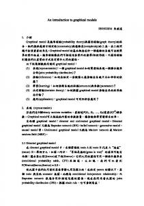


![[PDF] Introduction to Finite Elements Read Full Book - Google Sites](https://m.moam.info/img/260x300/pdf-introduction-to-finite-elements-read-full-book_647737f0097c4786708b7745.jpg)